Learning Theory Core
Empirical Risk Minimization
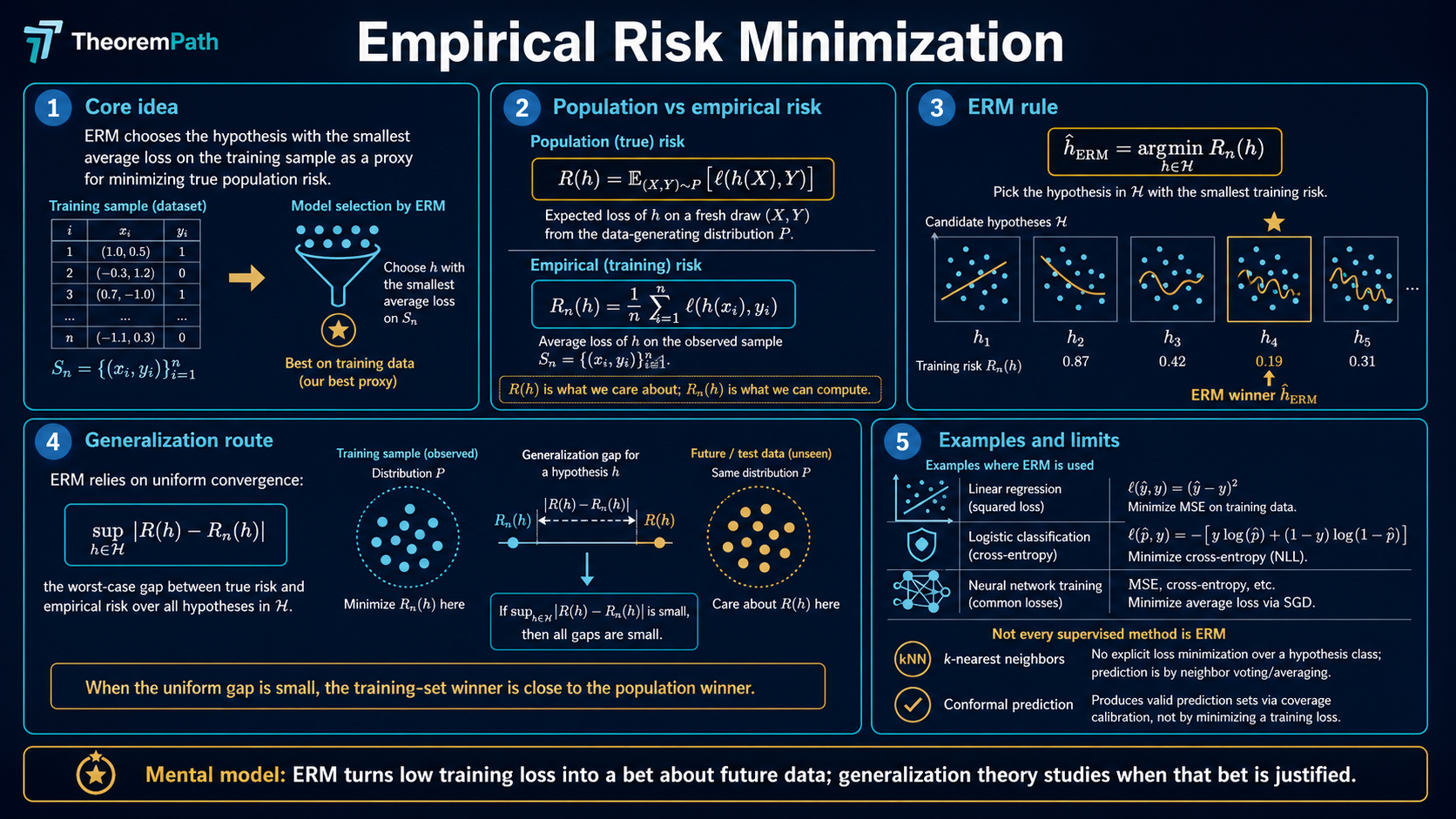
The foundational principle of statistical learning: minimize average loss on training data as a proxy for minimizing true population risk.
Prerequisites
Why This Matters
Many core supervised learning methods are empirical risk minimizers, or regularized variants thereof. When you train a neural network by minimizing cross-entropy loss on a training set, you are doing ERM. When you fit a linear regression by minimizing squared error, you are doing ERM. Other supervised methods sit outside the ERM frame: -nearest neighbors and Nadaraya-Watson kernel regression are local averaging rules with no global empirical-risk objective; full Bayesian posterior predictives average over a posterior rather than minimize a fixed loss; conformal prediction wraps a base learner and is calibrated on hold-out data instead of fitted by minimization. ERM is the dominant frame, not a universal one.
Hide overviewShow overview
Understanding ERM is the first step toward understanding why learning from data works at all, and where it fails.
Mental Model
Imagine you want to find a function that predicts well on future, unseen data. You cannot directly optimize over data you have not seen. So instead, you optimize over the data you have: your training set. And hope that good performance on training data translates to good performance on new data.
ERM formalizes this hope. The central question of learning theory is: when and why does this hope actually work?
Formal Setup and Notation
Let be an input space and an output space. Let be an unknown probability distribution over .
We have a loss function measuring prediction quality.
Notation reconciliation. TheoremPath uses for population risk and for empirical risk. Shalev-Shwartz and Ben-David use and respectively, with the second subscript encoding the realizable target. The statements coincide when the loss is 0-1 and is the labeling function: matches , and matches on training data labelled by . We use the SSBD notation when the realizability assumption is the analytical anchor; otherwise the form. The proof structure is the same; only the symbols change.
The phrase inductive bias from SSBD refers to the prior choice of hypothesis class that constrains the search space before any data is seen. Restricting is what protects ERM from overfitting on finite samples; the realizability assumption and the choice of class together determine when the protection is enough.
Population Risk
The population risk (or true risk) of a hypothesis is:
This is the quantity we actually want to minimize, but we cannot compute it directly because is unknown.
Empirical Risk
Given a training sample drawn i.i.d. from , the empirical risk is:
This is computable. It is the average loss on training data.
Empirical Risk Minimization
Given a hypothesis class , the ERM principle selects:
The key question: when is close to ?
Core Definitions
The generalization gap is the difference between population risk and empirical risk:
If this gap is small uniformly over all , then minimizing empirical risk also approximately minimizes population risk.
The approximation error is:
where is the Bayes risk. This measures how well the best hypothesis in can do, regardless of sample size.
The estimation error is:
This is what ERM theory actually controls.
Main Theorems
ERM Generalization via Uniform Convergence
Statement
If is finite and the loss is bounded in , then for any , with probability at least over the draw of :
Intuition
The bound says: if the hypothesis class is not too large (measured by ) and the sample is large enough, then empirical risk uniformly approximates population risk. The ERM hypothesis therefore has population risk close to the best in class.
Proof Sketch
Apply Hoeffding's inequality to each to get with probability . Then take a union bound over all hypotheses. Solve for .
Why It Matters
This is the simplest generalization bound in learning theory. It shows why ERM works for finite hypothesis classes. The dependence on rather than is crucial. It means the sample complexity grows only logarithmically in the number of hypotheses.
Failure Mode
This bound is vacuous for infinite hypothesis classes (e.g., all linear classifiers). You need more sophisticated complexity measures: VC dimension, Rademacher complexity, or covering numbers.
Lean-verified finite-class ERM tail
The Lean proof covers the finite-class Hoeffding chain: pointwise tail, finite-class union bound, closed-form rearrangement, sample-complexity bound, and ERM oracle inequality composed into a single excess-risk tail statement. Broader ERM claims for infinite or algorithm-specific hypothesis families stay source-checked until matching Lean statements are present.
Finite-class Hoeffding ERM excess-risk tail (Lean-verified)
Statement
For a finite nonempty hypothesis class with iid loss bounded in , an exact ERM hypothesis chosen on the empirical risk, and a best-in-class hypothesis , if
then
Proof Sketch
Apply the closed-form Hoeffding tail to the uniform deviation, then the
ERM oracle inequality , then
algebra on the bad event. The Lean proof is in
TheoremPath.LearningTheory.ERMGeneralization.finiteClass_hoeffding_exactERM_excessRisk_tail
(see the Lean manifest entry
claim:empirical-risk-minimization::finite-class-hoeffding-erm-excess-risk-tail).
The chain depends only on propext, Classical.choice, and Quot.sound.
Failure Mode
Lean-verified finite-class Hoeffding ERM excess-risk tail. This does not verify VC bounds, Rademacher bounds, infinite hypothesis classes, or generic PAC learnability. The page-level claim that "ERM works" still requires source review for the standard textbook treatment; the bound above is one specific tail statement on one specific hypothesis class shape.
Finite-class Hoeffding approximate-ERM excess-risk tail (Lean-verified)
Statement
Same setup as above but with only an approximate ERM with optimization slack (i.e., for all ). Then
Proof Sketch
The optimization slack enters additively from the approximate-ERM
oracle inequality .
Same Hoeffding tail as the exact case. Lean proof:
TheoremPath.LearningTheory.ERMGeneralization.finiteClass_hoeffding_approxERM_excessRisk_tail
(manifest entry
claim:empirical-risk-minimization::finite-class-hoeffding-approx-erm-excess-risk-tail).
Failure Mode
Same scope limits as the exact-ERM tail. Tying to a concrete optimization algorithm (e.g., SGD convergence rate) is a separate verification step that has not been done.
Effective-Growth VC-Style ERM Excess-Risk Tail
Statement
For a hypothesis class with effective-class cardinality bounded by the Sauer-Shelah growth function (for both and ), -bounded loss, iid sample , and any exact ERM :
Chains the deterministic ERM inequality (excess risk uniform deviation) with the VC-style two-sided uniform deviation bound. The leading term scales as .
Intuition
This is the standard VC sample-complexity theorem for ERM, expressed through the Rademacher route: Sauer-Shelah, Massart, Rademacher symmetrization, Azuma concentration, and ERM oracle inequality. The parameter plays the role of the VC dimension. For generic real-valued losses, the user supplies the effective-growth assumption. For binary classifiers with 0-1 loss, the binary-class VC bridge is now Lean-verified and closes that effective-loss-pattern step.
Failure Mode
The Azuma constant () is a factor of 4 looser than the sharp McDiarmid constant. The theorem applies only to finite hypothesis classes with bounded loss. The broader project has separate Lean support for the one-Lipschitz contraction lemma, but this ERM tail still does not prove infinite-class ERM or the full PAC-learnability equivalence.
Proof Ideas and Templates Used
The proof of the finite-class ERM bound uses two standard tools:
- Hoeffding's inequality: to control the deviation of the empirical mean from the true mean for a single hypothesis
- Union bound: to extend the guarantee from a single hypothesis to all hypotheses in the class simultaneously
This "Hoeffding + union bound" pattern is the simplest proof template in learning theory. It breaks for infinite classes because the union bound over uncountably many hypotheses gives infinity.
Canonical Examples
Finite binary classifiers
Suppose contains 1000 binary classifiers and we use 0-1 loss. With training examples and :
So the ERM hypothesis has population risk within about 2.3% of its training risk.
Memorization is the prototypical ERM failure
Take , binary labels , and a noisy target: (pure noise, Bayes risk ). Let be the class of all functions .
Draw training points . Define the memorizing hypothesis:
Then exactly: every training point is classified correctly.
But under any continuous distribution on , a freshly drawn hits a training with probability zero, so almost surely. The population risk is:
The empirical risk is zero; the population risk is the Bayes risk. The gap is , which is the worst possible value for binary 0-1 loss. ERM picks because it achieves , but the choice is useless on new data.
The fix is not "pick a different ERM"; it is to constrain so memorizing functions are excluded. The finite-class bound above shows that is the price for this constraint when is finite. The class of all functions has on a continuous , so the bound is vacuous and overfitting is unavoidable. This is exactly when VC dimension and Rademacher complexity take over.
Common Confusions
ERM is not the same as training loss minimization
ERM minimizes over a fixed hypothesis class . In practice, when you train a neural network, the class is parameterized and the optimization landscape matters. The ERM framework abstracts away optimization difficulty and asks: if you could find the exact minimizer, would it generalize? Real training adds optimization error on top of the estimation error ERM theory controls.
Small training loss does not imply small test loss
A model can memorize the training set (achieving zero empirical risk) while having terrible population risk. This happens when is too rich relative to . The generalization bound tells you when you can trust low training risk as a signal of low population risk.
Training loss and training error are not the same
In classification you typically optimize a convex surrogate loss (cross-entropy, hinge, logistic) while caring about the 0-1 classification error. "Minimizing training loss" (surrogate) and "minimizing training error" (0-1) are not equivalent. The connection is classification-calibration: a surrogate is calibrated if and only if minimizing its population risk implies minimizing the 0-1 population risk (Bartlett, Jordan, McAuliffe 2006). Cross-entropy, hinge, and logistic are calibrated; squared loss on targets is calibrated for binary classification; but not every convex surrogate is. Pages that use "training loss" and "training error" interchangeably are eliding this distinction.
Summary
- Population risk is what you want to minimize; empirical risk is what you can compute
- The generalization gap must be controlled uniformly
- For finite : gap scales as
- Total excess risk = approximation error + estimation error
- Richer reduces approximation error but increases estimation error. This is the bias-variance tradeoff
Exercises
Problem
Suppose has 100 hypotheses and the loss is bounded in . How many samples do you need so that with probability at least 0.95, the uniform convergence gap is at most 0.1?
Problem
Why can't you apply the finite-class ERM bound to the class of all linear classifiers in ? What goes wrong, and what tool do you need instead?
Related Comparisons
References
Canonical:
- Shalev-Shwartz & Ben-David, Understanding Machine Learning, Chapter 2-4
- Vapnik, Statistical Learning Theory (1998), Chapters 1-4
- Boucheron, Lugosi, Massart, Concentration Inequalities (2013), Chapter 4
Current:
- Mohri, Rostamizadeh, Talwalkar, Foundations of Machine Learning (2018), Chapter 2
- Wainwright, High-Dimensional Statistics (2019), Chapters 4-6
- Bartlett, Jordan, McAuliffe, "Convexity, Classification, and Risk Bounds," JASA (2006), arXiv:math/0508276 — classification-calibration of convex surrogate losses
- Bartlett, Long, Lugosi, Tsigler, "Benign overfitting in linear regression," PNAS 117 (2020), arXiv:1906.11300 — interpolating ERM solutions can still generalize when the spectrum decays appropriately
- Belkin, Hsu, Ma, Mandal, "Reconciling modern machine-learning practice and the classical bias-variance trade-off," PNAS 116 (2019), arXiv:1812.11118 — empirical "double descent" curves for ERM beyond the interpolation threshold
Next Topics
The natural next steps from ERM:
- Uniform convergence: the general framework for proving ERM works
- VC dimension: controlling complexity of infinite hypothesis classes
- Rademacher complexity: data-dependent complexity measurement
Last reviewed: April 26, 2026
Canonical graph
Required before and derived from this topic
These links come from prerequisite edges in the curriculum graph. Editorial suggestions are shown here only when the target page also cites this page as a prerequisite.
Required prerequisites
10- Common Inequalitieslayer 0A · tier 1
- Common Probability Distributionslayer 0A · tier 1
- Law of Large Numberslayer 0B · tier 1
- Maximum Likelihood Estimation: Theory, Information Identity, and Asymptotic Efficiencylayer 0B · tier 1
- Concentration Inequalitieslayer 1 · tier 1
Derived topics
13- Hypothesis Classes and Function Spaceslayer 2 · tier 1
- Overfitting and Underfittinglayer 2 · tier 1
- Realizability Assumptionlayer 2 · tier 1
- Uniform Convergencelayer 2 · tier 1
- VC Dimensionlayer 2 · tier 1
+8 more on the derived-topics page.
Graph-backed continuations