Algorithmic Stability

Why This Matters

The classical approach to generalization, uniform convergence via VC dimension or Rademacher complexity, analyzes the hypothesis class without regard to which algorithm selects a hypothesis from it. This is both a strength (algorithm-independent) and a weakness (cannot explain why specific algorithms generalize better than others on the same class).

Hide overviewShow overview

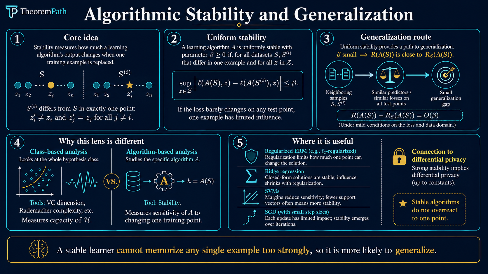
Algorithmic stability takes the opposite approach. It asks: how sensitive is the algorithm's output to perturbations of the training data? If replacing one training example barely changes the learned hypothesis, then the algorithm cannot be overfitting to any particular example, and generalization follows.

This perspective is essential for understanding modern ML: it explains why regularized ERM generalizes, provides the tightest known bounds for many algorithms (SVMs, ridge regression, stochastic gradient descent), and connects to differential privacy.

Mental Model

Imagine running your learning algorithm on a dataset $S$, then replacing one example $(x_i, y_i)$ with a fresh draw $(x_i', y_i')$ from the same distribution. If the resulting hypothesis barely changes, in the sense that its loss on any point changes by at most $\beta$, then the algorithm is $\beta$-uniformly stable.

The intuition is: if no single example has too much influence, then the algorithm is not memorizing individual examples, and therefore the training loss is a reliable estimate of the test loss.

Formal Setup and Notation

Let $\mathcal{A}$ be a (possibly randomized) learning algorithm that takes a training set $S = \{z_1, \ldots, z_n\}$ where $z_i = (x_i, y_i)$ drawn i.i.d. from $\mathcal{D}$, and outputs a hypothesis $\mathcal{A}(S)$.

Let $S^{(i)}$ denote the dataset obtained by replacing the $i$-th example $z_i$ with an independent copy $z_i'$ drawn from $\mathcal{D}$:

$S^{(i)} = \{z_1, \ldots, z_{i-1}, z_i', z_{i+1}, \ldots, z_n\}$

Definition

Uniform Stability$\beta \text{-stable}$

An algorithm $\mathcal{A}$ is $\beta$-uniformly stable (with respect to loss $\ell$) if and only if for all datasets $S$ of size $n$ and all indices $i$:

$\sup_z |\ell(\mathcal{A}(S), z) - \ell(\mathcal{A}(S^{(i)}), z)| \leq \beta$

That is, replacing any single training point changes the loss on any test point by at most $\beta$.

Definition

Hypothesis Stability

A weaker notion: $\mathcal{A}$ has hypothesis stability $\beta$ if and only if:

$\mathbb{E}_{S, z_i'}[|\ell(\mathcal{A}(S), z_i) - \ell(\mathcal{A}(S^{(i)}), z_i)|] \leq \beta$

This only requires the change to be small on average and at the replaced point. It is weaker than uniform stability but still implies generalization.

Definition

Generalization Gap (Stability Perspective)

The expected generalization gap is:

$\mathbb{E}_S[R(\mathcal{A}(S)) - \hat{R}_n(\mathcal{A}(S))]$

where $R(h) = \mathbb{E}_z[\ell(h, z)]$ is the population risk and $\hat{R}_n(h) = \frac{1}{n}\sum_{i=1}^n \ell(h, z_i)$ is the empirical risk. Stability directly controls this quantity.

Main Theorems

Theorem

Uniform Stability Implies Generalization

Statement

If $\mathcal{A}$ is $\beta$-uniformly stable, then the expected generalization gap satisfies:

$|\mathbb{E}_S[R(\mathcal{A}(S)) - \hat{R}_n(\mathcal{A}(S))]| \leq \beta$

Moreover, with probability at least $1 - \delta$ over the draw of $S$ (two-sided form):

$|R(\mathcal{A}(S)) - \hat{R}_n(\mathcal{A}(S))| \leq \beta + (2n\beta + M)\sqrt{\frac{\ln(2/\delta)}{2n}}$

Bousquet and Elisseeff (2002, Theorem 12) state the one-sided version with $\ln(1/\delta)$. The two-sided form above follows by a union bound over the two tails, which replaces $\ln(1/\delta)$ with $\ln(2/\delta)$.

Intuition

The expected bound follows from a leave-one-out symmetry argument. By linearity, the expected generalization gap equals the average (over $i$) of $\mathbb{E}[\ell(\mathcal{A}(S), z_i') - \ell(\mathcal{A}(S), z_i)]$. Since $z_i$ and $z_i'$ have the same distribution, swapping them does not change the expectation. Stability means the algorithm barely notices the swap, so the gap is bounded by $\beta$.

Proof Sketch

Define $\Phi(S) = R(\mathcal{A}(S)) - \hat{R}_n(\mathcal{A}(S))$. We show $\mathbb{E}[\Phi]$ is small and $\Phi$ concentrates.

For the expectation: write $R(\mathcal{A}(S)) = \mathbb{E}_{z'}[\ell(\mathcal{A}(S), z')]$ and $\hat{R}_n(\mathcal{A}(S)) = \frac{1}{n}\sum_i \ell(\mathcal{A}(S), z_i)$. Since $z_i' \sim \mathcal{D}$ independently, $\mathbb{E}[\ell(\mathcal{A}(S), z_i')] = \mathbb{E}[\ell(\mathcal{A}(S^{(i)}), z_i)]$ by the symmetry of $z_i$ and $z_i'$. Stability gives $|\ell(\mathcal{A}(S), z_i) - \ell(\mathcal{A}(S^{(i)}), z_i)| \leq \beta$, so $|\mathbb{E}[\Phi]| \leq \beta$.

For concentration: replacing $z_i$ with $z_i'$ to form $S^{(i)}$ changes $\Phi(S) = R(\mathcal{A}(S)) - \hat R_n(\mathcal{A}(S))$ by at most $2\beta + M/n$. The two sources of change are:

1. The risk term $R(\mathcal{A}(S))$ depends on $S$ only through $\mathcal{A}(S)$, and $\beta$-stability implies $|\ell(\mathcal{A}(S),z) - \ell(\mathcal{A}(S^{(i)}),z)| \le \beta$ for any $z$, so $|R(\mathcal{A}(S)) - R(\mathcal{A}(S^{(i)}))| \le \beta$.
2. The empirical-risk term changes by at most $\beta$ on the $n-1$ unchanged points (again by stability) and by at most $M/n$ on the single replaced point (the loss is bounded by $M$, so its $\frac{1}{n}$-weighted contribution shifts by at most $M/n$).

Adding the two contributions gives the bounded-difference constant $2\beta + M/n$. Apply McDiarmid with these bounded differences across the $n$ coordinates.

Why It Matters

This theorem gives a completely different path to generalization bounds. Instead of measuring the complexity of $\mathcal{H}$, you measure the sensitivity of $\mathcal{A}$. For regularized algorithms, $\beta$ often decreases as regularization increases, giving a direct explanation of the regularization-generalization connection.

Failure Mode

Uniform stability requires the worst-case change over all possible datasets and all possible replacement points to be small. Many algorithms (including unregularized ERM over rich classes) are not uniformly stable. The bound is vacuous if $\beta$ is large.

report a correction →

Theorem

Bousquet-Elisseeff: Regularized ERM is Stable

Statement

Convention. A function $f$ is $\mu$-strongly convex if and only if $f - (\mu/2)\|\cdot\|^2$ is convex (equivalently, $\nabla^2 f \succeq \mu I$ for twice-differentiable $f$). Under this convention, $\|\cdot\|_2^2$ is $2$-strongly convex, and $\lambda\|\cdot\|_2^2$ is $2\lambda$-strongly convex.

If the loss $\ell(h, z)$ is $L$-Lipschitz in $h$ and the regularized ERM objective $\hat{R}_n(h) + \Omega(h)$ has a $\mu$-strongly convex regularizer $\Omega$, then the regularized ERM algorithm is $\beta$-uniformly stable with:

$\beta = \frac{L^2}{2\mu n}$

This matches Bousquet and Elisseeff (2002, Theorem 22) directly. Shalev-Shwartz and Ben-David (2014, Corollary 13.6) use a different convention (calling $\|\cdot\|^2$ itself $1$-strongly convex), which yields the equivalent bound $2\rho^2/(\lambda n)$ with $\rho = L$ and $\lambda$ the regularization weight.

Intuition

Strong convexity means the objective has a unique minimizer, and that minimizer moves continuously (in fact, Lipschitz-continuously) when you perturb the data. Replacing one example out of $n$ perturbs the objective by $O(1/n)$, and the strong convexity constant $\mu$ determines how much the minimizer moves per unit of perturbation. The result is stability $O(1/(\mu n))$.

Proof Sketch

Let $h_S$ and $h_{S^{(i)}}$ be the minimizers of $F_S(h) = \hat{R}_n(h) + \Omega(h)$ and the analogous $F_{S^{(i)}}$. By optimality:

$F_S(h_S) \leq F_S(h_{S^{(i)}}), \qquad F_{S^{(i)}}(h_{S^{(i)}}) \leq F_{S^{(i)}}(h_S)$

Adding these, only the two loss terms at index $i$ survive; $L$-Lipschitzness of $\ell$ bounds their contribution by $2L\|h_S - h_{S^{(i)}}\|/n$. Strong convexity of $F_S$ (inherited from $\Omega$) at its minimizer $h_S$ gives

$F_S(h_{S^{(i)}}) - F_S(h_S) \geq (\mu/2)\|h_S - h_{S^{(i)}}\|^2$

and similarly for $F_{S^{(i)}}$. Combining yields $\mu \|h_S - h_{S^{(i)}}\|^2 \leq 2L\|h_S - h_{S^{(i)}}\|/n$, so

$\|h_S - h_{S^{(i)}}\| \leq \frac{2L}{\mu n}$

Lipschitzness of the loss gives $|\ell(h_S, z) - \ell(h_{S^{(i)}}, z)| \leq L \cdot 2L/(\mu n) = 2L^2/(\mu n)$. Taking the max over the two sides of the swap (equivalently, using a sharper one-sided argument via first-order optimality conditions) gives the tighter constant $\beta = L^2/(2\mu n)$ stated above. See Bousquet-Elisseeff (2002), proof of Theorem 22, for the argument that avoids the factor-of-4 loss.

Why It Matters

This is the theorem that explains why regularization helps generalization from a stability perspective. For ridge regression ($\lambda\|w\|^2$-regularized least squares), the regularizer is $2\lambda$-strongly convex, giving stability $O(1/(\lambda n))$ and therefore a generalization bound of $O(1/(\lambda n))$. Combined with the approximation error (which grows with $\lambda$), you get the classical bias-variance tradeoff derived purely from stability.

Failure Mode

Requires strong convexity of the regularizer and Lipschitzness of the loss. Without regularization ($\lambda = 0$), the bound is vacuous. Non-convex problems (neural networks) are not directly covered, though SGD-specific stability analyses exist.

report a correction →

The diagram makes the $\beta = L^2/(2\mu n)$ scaling concrete. With $L = 1$ fixed, three regularization strengths trace out three $1/n$ decay curves, vertically separated by $1/\mu$. The horizontal threshold at $\beta = 0.05$ marks where the bound becomes operationally non-vacuous: $\mu = 0.01$ requires $n \geq 1000$ to clear it, $\mu = 0.1$ requires $n \geq 100$, and $\mu = 1.0$ requires only $n \geq 10$. This is the regularization side of the bias-variance tradeoff in raw form: heavier $\mu$ buys stability cheaper in $n$ but pays in approximation error not shown here.

The McDiarmid Connection

The high-probability bound in the stability theorem uses McDiarmid's inequality (the bounded differences inequality). The key observation:

If $\mathcal{A}$ is $\beta$-uniformly stable, then the generalization gap $\Phi(S) = R(\mathcal{A}(S)) - \hat{R}_n(\mathcal{A}(S))$ satisfies a bounded differences condition: replacing any $z_i$ changes $\Phi$ by at most

$|\Phi(S) - \Phi(S^{(i)})| \leq 2\beta + M/n$

The $2\beta$ comes from the change in $R(\mathcal{A}(S))$ (stability applied to the test loss), and $M/n$ comes from the direct change in $\hat{R}_n$ when one of its $n$ terms changes.

McDiarmid's inequality then gives: $\mathbb{P}(|\Phi - \mathbb{E}[\Phi]| \geq t) \leq 2\exp(-2t^2/(n(2\beta + M/n)^2))$.

Canonical Examples

Example

Ridge Regression

Ridge regression minimizes

$$\frac{1}{n}\sum_{i=1}^n (y_i - w^\top x_i)^2 + \lambda \|w\|_2^2.$$

The squared loss is $L$-Lipschitz in $w$ on the relevant ball when features are bounded ($\|x\| \leq B$), with effective $L = O(B)$ after a standard a priori bound on $\|w\|$. The regularizer $\lambda\|w\|_2^2$ is $\mu$-strongly convex with $\mu = 2\lambda$. Applying the theorem:

$\beta = \frac{L^2}{2\mu n} = \frac{L^2}{4\lambda n}$

With $n = 1000$, $L = B = 1$, $\lambda = 0.01$: $\beta \approx 0.025$. The expected generalization gap is at most about $2.5\%$.

Example

Regularized SVM

The soft-margin SVM with regularization $\lambda\|w\|^2$ and hinge loss $\ell(w, (x,y)) = \max(0, 1 - y w^\top x)$ is uniformly stable with $\beta = 1/(4\lambda n)$ (hinge loss is $1$-Lipschitz when $\|x\| \leq 1$, regularizer has $\mu = 2\lambda$, so $\beta = L^2/(2\mu n) = 1/(4\lambda n)$). The looser quote $\beta = 1/(2\lambda n)$ also appears in the literature; both forms are correct under different bookkeeping conventions.

Stability theory itself originated earlier with Devroye and Wagner (1979) for $k$-nearest-neighbor and other potential-function rules. SVMs and other regularized convex methods became the headline application in Bousquet and Elisseeff (2002).

SGD Stability (Hardt, Recht, Singer 2016)

Classical Bousquet-Elisseeff covers the exact minimizer of a strongly convex regularized objective. Hardt, Recht, and Singer (2016, arXiv:1509.01240) extend the framework to the iterates of stochastic gradient descent, without assuming a regularizer.

Theorem

SGD Stability: Smooth Convex Case

Statement

For an $L$-Lipschitz, $\beta$-smooth, convex loss, SGD with step sizes $\eta_t \leq 2/\beta$ run for $T$ steps is $\epsilon_{\text{stab}}$-uniformly stable with:

$\epsilon_{\text{stab}} \leq \frac{2L^2}{n} \sum_{t=1}^T \eta_t$

In particular, $T$ steps of constant step size $\eta$ give $\epsilon_{\text{stab}} = O(L^2 \eta T / n)$.

Intuition

The gradient-update map $w \mapsto w - \eta \nabla \ell(w, z)$ is $1$-expansive when $\eta \leq 2/\beta$ and the loss is convex: replacing one training example and running the same SGD trajectory cannot inflate the iterate gap faster than the single perturbed step introduces. The per-step perturbation is at most $\eta L$ with probability $1/n$ (the swap hits the current example). Summing over $T$ steps gives the bound.

Why It Matters

Two operational consequences. First, early stopping acts as a regularizer via stability: fewer steps means smaller $\sum_t \eta_t$ means tighter generalization bound. Second, long training with constant step size can hurt generalization even if training loss is small: the stability term grows linearly in $T$, so at some point it dominates any training-loss improvement.

Failure Mode

Non-expansivity requires $\eta_t \leq 2/\beta$ and convexity. Past the smoothness-compatible step size, gradient updates can be expansive and the argument breaks.

report a correction →

For smooth non-convex losses (the realistic deep-learning regime), Hardt-Recht-Singer show that with decaying step size $\eta_t = c/t$, SGD is uniformly stable with:

$\epsilon_{\text{stab}} = O\!\left(\frac{T^{1 - 1/(c\beta + 1)}}{n}\right)$

where $\beta$ is the smoothness constant. The exponent $1 - 1/(c\beta + 1) \in (0, 1)$ gives a sub-linear growth in $T$: the bound is non-vacuous for moderate $T/n$ but degrades as $T$ grows. This is a formal version of "don't train forever."

Watch Out

SGD stability assumes smoothness, not convexity

A frequent reading error: the non-convex bound is presented without the convex assumption, but smoothness ($\beta$-Lipschitz gradients) is still required. Non-smooth losses like hinge or ReLU-network losses are not directly covered; extensions exist but require additional assumptions (e.g., subgradient bounds, sampling without replacement analyses).

Differential Privacy Connection

$(\epsilon, \delta)$-differential privacy and uniform stability are closely related. Intuitively, DP bounds the distributional effect of swapping one training point on the output distribution; stability bounds its effect on loss values. For loss bounded in $[0, M]$, $(\epsilon, \delta)$-DP implies uniform stability at scale roughly $M(e^{\epsilon} - 1) + M\delta$, which is $O(M\epsilon)$ for small $\epsilon$.

Two constructions give stability by design:

• Output perturbation. Train a regularized ERM, add calibrated Gaussian or Laplace noise to the weights. The noise scale gives both the DP guarantee and an explicit stability bound.
• DP-SGD (Abadi et al., 2016, arXiv:1607.00133). Clip per-example gradients to norm $C$, add Gaussian noise $\mathcal{N}(0, \sigma^2 C^2 I)$ to each aggregated minibatch gradient. The moments accountant tracks the cumulative $(\epsilon, \delta)$ over $T$ steps. The same noise that buys privacy also buys stability, and therefore generalization.

This bridge matters for modern ML: when you cannot prove stability directly (non-convex, large models), DP noise offers a constructive path. The price is utility loss proportional to the noise scale.

Convention Equivalence: BE vs SSBD

Two common definitions of stability appear in the literature. They agree up to small constants; the distinction is worth making explicit because papers quote bounds in whichever convention is convenient.

• Bousquet-Elisseeff 2002 (BE). Worst-case, pointwise: $\sup_{z, S, i}\; |\ell(\mathcal{A}(S), z) - \ell(\mathcal{A}(S^{(i)}), z)| \leq \beta$.
• Shalev-Shwartz-Ben-David 2014 (SSBD), Chapter 13. In-expectation, replace-one: $\mathbb{E}_{S, z_i'}[\ell(\mathcal{A}(S), z_i') - \ell(\mathcal{A}(S^{(i)}), z_i')] \leq \epsilon_{\text{stab}}(n)$.

For loss bounded in $[0, M]$, BE $\beta$-uniform stability implies SSBD $\epsilon_{\text{stab}} \leq \beta$ immediately (expectation of a quantity bounded by $\beta$ is bounded by $\beta$). The reverse does not hold in general: in-expectation stability is strictly weaker.

Leave-one-out vs replace-one. Some sources define stability via the leave-one-out dataset $S^{\setminus i} = \{z_1, \ldots, z_{i-1}, z_{i+1}, \ldots, z_n\}$ of size $n-1$ instead of the replace-one set $S^{(i)}$ of size $n$. A one-line algebraic bridge:

$|\ell(\mathcal{A}(S), z) - \ell(\mathcal{A}(S^{\setminus i}), z)| \leq |\ell(\mathcal{A}(S), z) - \ell(\mathcal{A}(S^{(i)}), z)| + |\ell(\mathcal{A}(S^{(i)}), z) - \ell(\mathcal{A}(S^{\setminus i}), z)|$

Each term on the right is controlled by the replace-one (or leave-one-out) stability at the appropriate sample size. For bounded loss the cost of switching conventions is at most a factor of $2$, and when $\beta(n)$ scales as $1/n$ (the common case) the swap changes the bound by at most $O(1/n^2)$, which is negligible next to the leading $O(1/n)$ stability term. PAC-Bayes and stability bounds both target the same generalization quantity via different perturbation models.

Common Confusions

Watch Out

Stability does NOT imply generalization in the converse direction

A common misconception: "if an algorithm generalizes, it must be stable." This is false. There exist algorithms with non-trivial risk guarantees that are not uniformly stable. The classical example is 1-nearest-neighbor: by Cover and Hart (1967), its asymptotic risk is at most twice the Bayes risk, yet it has poor uniform stability because changing one training example can flip predictions in its Voronoi cell. Note that 1-NN is not strongly consistent in general; strong consistency requires $k$-NN with $k \to \infty$ and $k/n \to 0$ (Stone, 1977). So "1-NN generalizes" should be read as "has a meaningful risk bound," not "converges to the Bayes classifier."

Stability is sufficient for generalization but not necessary. The relationship is one-directional.

Watch Out

Uniform stability is a strong requirement

Uniform stability requires the loss change to be bounded for every dataset and every test point. This is much stronger than average-case guarantees. Many practical algorithms satisfy weaker notions (hypothesis stability, on-average stability) but not uniform stability. The Bousquet-Elisseeff framework specifically addresses regularized ERM, which is one of the few settings where uniform stability holds cleanly.

Watch Out

Stability bounds and uniform convergence bounds are not competing

Stability bounds and complexity-based bounds (VC, Rademacher) are complementary, not contradictory. They analyze different aspects of learning: complexity bounds measure the class, stability bounds measure the algorithm. For a given algorithm on a given class, one may be tighter than the other. The right tool depends on the situation.

Why Stability Explains Regularized ERM

The Bousquet-Elisseeff theorem gives a clean narrative:

1. Unregularized ERM on a rich class is typically not stable. The minimizer can jump drastically when one example changes, because there are many near-optimal hypotheses.

2. Adding regularization (e.g., $\lambda\|w\|^2$) makes the objective strongly convex, which forces a unique minimizer that varies smoothly with the data.

3. Stronger regularization (larger $\lambda$) gives better stability ($\beta \propto 1/\lambda$) and therefore better generalization, but worse approximation (bias). This is exactly the bias-variance tradeoff.

4. Optimal $\lambda$ balances stability (generalization) against approximation error, recovering the classical $O(1/\sqrt{n})$ rate.

Exercises

ExerciseCore

Problem

Suppose an algorithm $\mathcal{A}$ is $\beta$-uniformly stable with $\beta = 1/n$. The loss is bounded in $[0, 1]$. What is the expected generalization gap? Give a high-probability bound with $\delta = 0.05$.

Hint

Reveal Solution

ExerciseAdvanced

Problem

Prove that unregularized ERM over the class of all linear classifiers in $\mathbb{R}^d$ (with 0-1 loss) is not uniformly stable. Construct an explicit example where replacing one training point causes the loss on some test point to change by $\Omega(1)$.

Hint

Reveal Solution

ExerciseAdvanced

Problem

For $\ell_2$-regularized logistic regression with regularization parameter $\lambda$, features bounded by $\|x\| \leq B$, what is the uniform stability parameter? The logistic loss is $\ell(w,(x,y)) = \log(1 + e^{-y w^\top x})$.

Hint

Reveal Solution

References

Canonical:

• Bousquet & Elisseeff, "Stability and Generalization" (2002), JMLR 2:499-526. Theorems 12 (high-probability bound) and 22 (regularized ERM stability).
• Shalev-Shwartz, Shamir, Srebro, Sridharan, "Learnability, Stability, and Uniform Convergence" (2010), JMLR 11:2635-2670. Shows that in stochastic convex optimization, stability characterizes learnability even in regimes where uniform convergence fails: a counterexample to the equivalence "learnability $\iff$ uniform convergence" that holds for binary classification.
• Shalev-Shwartz & Ben-David, Understanding Machine Learning (2014), Chapter 13 (stability and regularization). Uses the convention where $\|\cdot\|^2$ is itself called $1$-strongly convex; bounds therefore appear with different constants than Bousquet-Elisseeff.
• Devroye & Wagner, "Distribution-Free Performance Bounds for Potential Function Rules" (1979), IEEE Trans. IT 25(5):601-604. The earliest stability-style analysis, predating the Bousquet-Elisseeff framework by two decades.

Current:

• Hardt, Recht, Singer, "Train faster, generalize better: Stability of stochastic gradient descent" (2016), ICML; arXiv:1509.01240. Shows that for $L$-Lipschitz, $\beta$-smooth, convex losses, SGD with step size $\eta_t \leq 2/\beta$ is uniformly stable with bound $(2L^2/n)\sum_t \eta_t$ after $T$ steps; in the strongly convex case the bound becomes dimension-free $O(1/n)$; for smooth non-convex losses with $\eta_t = c/t$, stability is $O(T^{1 - 1/(c\beta + 1)}/n)$.
• Abadi, Chu, Goodfellow, McMahan, Mironov, Talwar, Zhang, "Deep Learning with Differential Privacy" (2016), CCS; arXiv:1607.00133. Introduces DP-SGD with per-example gradient clipping, Gaussian noise, and the moments accountant. The construction provides $(\epsilon, \delta)$-DP and, via the DP-to-stability implication, explicit generalization bounds.
• Boucheron, Lugosi, Massart, Concentration Inequalities (2013), Chapter 6 (McDiarmid's inequality and bounded differences).

Next Topics

The natural next step from algorithmic stability:

• Implicit bias and modern generalization: how stability and implicit regularization explain deep learning