Statistical Estimation
Maximum Likelihood Estimation: Theory, Information Identity, and Asymptotic Efficiency
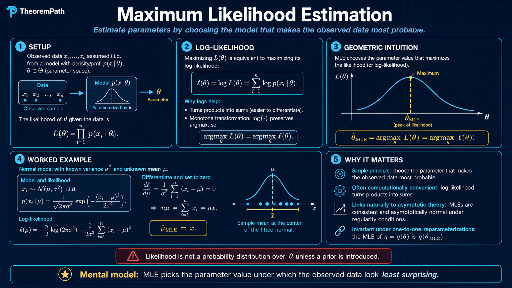
MLE: pick the parameter that maximizes the likelihood of observed data. Score function, Bartlett identities, regularity conditions, consistency, asymptotic normality, Wilks' theorem, Cramér-Rao efficiency, exponential families, QMLE under misspecification, and the bridge to deep-learning negative log-likelihood training.
Prerequisites
Why This Matters
Maximum likelihood estimation is the workhorse of parametric inference, and almost every modern training objective is a likelihood in disguise. Train a logistic regression by minimizing cross-entropy loss and you are running MLE on a Bernoulli/categorical model. Fit a Gaussian mixture model and you are running MLE via EM. Train a language model by minimizing perplexity and you are running MLE on a categorical sequence model. Even modern generative models (variational autoencoders, normalizing flows, autoregressive transformers) train against the negative log-likelihood (NLL) or a tractable bound on it.
Hide overviewShow overview
Five questions decide whether the MLE is the right tool for a given problem:
- Does it converge to the truth? Consistency: under identifiability and standard regularity (Cramér 1946; Wald 1949).
- How accurate is it? Asymptotic normality: under Cramér-type regularity.
- Can any unbiased estimator do better? Cramér-Rao: no regular unbiased estimator has smaller variance than . The MLE attains this bound asymptotically.
- What if the model is wrong? White's QMLE: the MLE converges to the least-false parameter , with sandwich variance replacing .
- What can we test? Wilks' theorem: under (with non-central under contiguous alternatives), so the likelihood-ratio statistic has a calibrated null distribution.
Each answer requires the information identity , which fails the moment regularity does, and recognizing those failures is what separates a working statistician from a textbook user.
Likelihood gives one geometric object and three equally important readings
Maximum likelihood picks the parameter where the log-likelihood peaks.
Optimization target
The MLE is the parameter value where the observed data has the largest joint density under the model.
Why logs matter
The log transform turns products into sums, making numerical optimization and asymptotic analysis possible.
ML translation
Cross-entropy, token negative log-likelihood, and many probabilistic deep-learning losses are MLE objectives in disguise.
Mental Model
You observe from with unknown . The MLE asks: which assigns the largest joint density to what you actually saw? Two equivalent framings:
- Pick the parameter under which your data is least surprising. Each datum contributes a log-likelihood ; the MLE maximizes the sum.
- Minimize empirical cross-entropy against the model. . This form is what most ML loss functions are: minimizing categorical cross-entropy or negative log-likelihood is exactly MLE. For discrete models with shared support, this also equals the information projection in Csiszár's sense, since the empirical entropy is -independent. For continuous-density models the empirical is a discrete mixture of point masses, so in the strict measure-theoretic sense; the KL framing then holds only as a formal/heuristic identity, while empirical cross-entropy minimization holds rigorously.
The log transform converts products into sums, which buys two things at once: numerical stability (no underflow on long sequences) and access to the law of large numbers and central limit theorem (sums of i.i.d. terms are exactly what asymptotic statistics is designed to handle). This single change turns finite-sample maximum-density into an asymptotic theory of estimators.
Formal Setup and Notation
Let be i.i.d. from where . The parametric family is the statistical model. The dominating measure is (Lebesgue on for continuous data, counting on for discrete data); is a density with respect to .
Likelihood Function
The likelihood function is
It is a function of with the data fixed. Despite looking like a density on the data space, is not a probability distribution over (it does not integrate to one over ). Bayesians multiply by a prior and renormalize to obtain a posterior; frequentists treat as the input to estimation and testing.
Log-Likelihood
The log-likelihood is
The log transform turns products into sums, which is required for the law of large numbers, the central limit theorem, and floating-point stability on long product chains.
Maximum Likelihood Estimator
The MLE is any measurable maximizer
When is open and is differentiable, solves the score equation where . The MLE may not exist (infinite or non-attained supremum), may not be unique (multimodal ), and may sit on the boundary of . Existence and uniqueness require structural assumptions (compactness of , concavity of , identifiability, or all three).
Score Function and Fisher Information
Score Function
The score function is the gradient of the log-density:
Under regularity (interchange of differentiation and integration), the score has mean zero at the true parameter:
The MLE satisfies , the empirical analog of .
Fisher Information
The (per-observation, expected) Fisher information at is
a positive semidefinite matrix. Under second-order regularity (twice differentiability of and a second-order interchange) it equals the negative expected Hessian:
For i.i.d. observations the total information is . Fisher information measures how sharply the log-likelihood concentrates around the truth: large means a steep peak (easy to estimate), small means a flat surface (hard to estimate).
Observed Fisher Information
The (data-dependent) observed Fisher information is
By the law of large numbers . In practice one reports as a finite-sample variance estimate; under misspecification does not equal the population and the sandwich form is needed (see QMLE below).
The Information Identity
The two formulas and are not separate definitions; they are equal under regularity, and the equality is the single most-used identity in likelihood theory. Bartlett (1953) generalized this to a family of cumulant identities obtained by repeated differentiation of .
Bartlett Identities (Information Equality)
Statement
Under regularity, the score has mean zero and Fisher information equals the negative expected Hessian:
Equivalently, , the second Bartlett identity.
Intuition
Differentiate once: . Differentiate again:
Since , this rearranges to . The identity is bookkeeping that turns one expression for into the other; the content is that you can interchange differentiation and integration.
Proof Sketch
Step 1 (first identity). Differentiate with respect to . Pass the derivative inside the integral (assumption). Use . Conclude .
Step 2 (second identity). Differentiate again. By the same interchange,
A cleaner path is to differentiate the score directly. From , differentiate:
Take expectation under , using from Step 1's interchange:
Since , this gives , equivalently .
Why It Matters
The information identity is the linchpin of three subsequent results:
- Asymptotic normality of the MLE uses to identify the variance.
- Cramér-Rao uses in the Cauchy-Schwarz step.
- Wilks' theorem uses both forms when expanding to second order.
When the identity fails (parameter on a boundary, support depending on , non-smooth ), every classical asymptotic for the MLE fails along with it, and you need M-estimator machinery (sandwich variance, cube-root rates, mixture- limits) instead.
Failure Mode
The interchange step requires more than two derivatives existing. Standard counterexamples: (1) Uniform with support depends on , so but ; the score is not even well-defined and the MLE is with rate , not . (2) Models with a discontinuity in at a -dependent threshold (change-point models) violate the same interchange; the MLE has a non-Gaussian limit at rate . (3) Mixture models on the boundary () make singular and the second identity meaningless.
Regularity Conditions
The asymptotic theorems below require the parametric family to be regular. The canonical Cramér-type list (van der Vaart 1998 Ch. 5; Lehmann-Casella 1998 Ch. 6):
- Identifiability: as measures.
- Common support: does not depend on .
- Interior: .
- Smoothness: is three times continuously differentiable in , with third derivatives uniformly bounded by an integrable envelope in a neighborhood of .
- Interchange: differentiation under the integral sign is valid through second order (justified by dominated convergence with the same envelope).
- Information: is finite and positive definite.
Le Cam (1970) replaced conditions 4-5 with the much weaker differentiability in quadratic mean (DQM): there exists a score-like vector such that in . DQM holds for all common parametric families and yields the same asymptotic normality without requiring three derivatives or an envelope. See asymptotic-statistics for the LAN treatment.
Main Theorems
Consistency of the MLE (Wald)
Statement
Under Wald's conditions, the MLE is consistent:
If is open (rather than compact), the same conclusion holds when is concave and is the unique maximizer of .
Intuition
The empirical log-likelihood per observation is a sample average of i.i.d. terms. By the law of large numbers, pointwise. The Kullback-Leibler inequality gives
with equality only when , i.e. (by identifiability) . So uniquely maximizes the limit objective. Under uniform convergence (Wald's compactness + envelope, or concavity), the maximizer of converges to the maximizer of , which is .
Proof Sketch
Step 1 (LLN). For each , by the strong law.
Step 2 (uniform convergence). Compactness + envelope yields (uniform LLN; van der Vaart Lemma 19.36 or Newey-McFadden Lemma 2.4).
Step 3 (KL identifies the max). for by Gibbs' inequality and identifiability.
Step 4 (argmax convergence). A standard argmax-continuity argument (van der Vaart Theorem 5.7) gives .
Why It Matters
Consistency is the minimum bar for any estimator and the prerequisite for asymptotic normality (which is local around ). The proof structure has three parts: LLN gives pointwise convergence; uniformity comes from compactness or concavity; KL identifies the maximizer. It is the template every modern consistency proof reuses (M-estimators, GMM, EM, deep learning's empirical loss).
Failure Mode
(1) Non-identifiability. Mixture models with label-switching: and give the same density. The KL gap collapses on the orbit, and the MLE is not consistent for any single labeling. (2) Boundary blow-up. In Gaussian mixtures, sending one component's variance to zero with its mean equal to a data point makes . The MLE does not exist; constrained or penalized variants are needed. (3) Neyman-Scott. Parameter dimension growing with (one mean per pair of observations, one shared variance) gives an inconsistent variance MLE. Profile or modified likelihoods recover consistency. (4) Misspecification. If is not in the model family, the MLE converges to the least-false parameter , not to any "true" (see QMLE below).
Asymptotic Normality of the MLE
Statement
Under regularity and consistency, the MLE is asymptotically normal:
Equivalently, for large . The variance is the Cramér-Rao lower bound, attained by the MLE in the limit.
Intuition
Taylor-expand the score equation around :
The first term, scaled by , is a CLT for an i.i.d. mean-zero sum with covariance (Bartlett identity I), so . The bracket converges in probability to (Bartlett identity II + LLN). Solving,
Proof Sketch
Step 1 (Taylor). Mean-value-expand the score: for some between and .
Step 2 (CLT). by the multivariate CLT (Bartlett identity I gives the variance).
Step 3 (LLN + consistency). by the uniform LLN plus continuity at and consistency of .
Step 4 (Slutsky). Combining steps 2 and 3,
Why It Matters
Asymptotic normality is the engine behind every classical inferential procedure built on the MLE: Wald confidence intervals , Wald hypothesis tests, model comparison via AIC and BIC (which use the asymptotic distribution of the maximized log-likelihood). The functional form also plugs straight into the delta method for any smooth , giving CIs for derived quantities (odds ratios, hazard ratios, predicted probabilities).
Failure Mode
Asymptotic normality fails in four canonical cases. (1) sits on the boundary of (variance equal to zero, mixture proportion equal to zero): the limit becomes a projection of a Gaussian onto a tangent cone (Self-Liang 1987). (2) Fisher information is singular (flat likelihood, weak identification): the rate slows below or the limit becomes non-Gaussian. (3) The model is misspecified: replace with the sandwich (QMLE, below). (4) Finite-sample concerns dominate, especially in high dimensions where the regime requires in many examples.
Wilks' Theorem (LRT Asymptotic χ²)
Statement
Let be the likelihood ratio comparing the constrained MLE under to the unconstrained MLE. Under the null,
where is the codimension of the null (number of restrictions). Under contiguous alternatives , the limit is non-central with non-centrality , where is the restricted block of Fisher information.
Intuition
Taylor-expand the log-likelihood around the unconstrained MLE:
The vector is asymptotically Gaussian, projected onto the orthogonal complement of the null tangent space (a -dimensional subspace). Quadratic forms of -dim Gaussians with the right covariance are exactly .
Proof Sketch
Step 1. Under regularity, and (projection onto the null tangent space in the Fisher metric).
Step 2. Second-order Taylor expansion of around gives (the gradient at is zero, the Hessian at converges to by Bartlett II).
Step 3. Substituting Step 1 into Step 2: the limit is , the squared Fisher norm of the projection of onto the orthogonal complement of . This equals . Substituting and choosing coordinates so that the orthogonal complement is the first axes gives .
Why It Matters
Wilks' theorem makes the likelihood-ratio test (LRT) practical: you can compute and compare to a critical value without ever computing Fisher information by hand. It is the basis for nested-model comparison in regression (drop predictors and the LRT has a null), in GLMs (deviance differences), in mixed models, in survival analysis (Cox PH), and in modern model selection (BIC penalty derives from the Wilks limit). The non-central result under contiguous alternatives gives the asymptotic power of the test; see the LRT vs Wald vs score equivalence in asymptotic-statistics.
Failure Mode
Wilks' fails on the same boundaries that asymptotic normality does. Self-Liang (1987) shows that on a parameter-space boundary the limit is a mixture of distributions (e.g., for testing in a mixed model the limit is ). Under non-identifiability (testing whether a mixture component is present, the famous "two-component vs. one-component" test) the limit is non-standard and depends on a nuisance parameter under the alternative (Davies 1977). Don't apply Wilks blindly when the null is on a boundary or weakly identified.
Cramér-Rao Lower Bound
Statement
Let be unbiased for . Then
In the multivariate case (), in the Loewner order. An estimator attaining the bound is called efficient. The MLE achieves the bound asymptotically (the previous theorem).
Intuition
Differentiating in gives where is the total score. Cauchy-Schwarz gives . The information sets the price tag on precision: each unit of Fisher information buys a unit of variance reduction.
Proof Sketch
Step 1. From , differentiate under the integral: for ; the i.i.d. case generalizes to .
Step 2. Since , .
Step 3. Cauchy-Schwarz: .
Step 4. Rearrange: .
Why It Matters
Cramér-Rao is the universal benchmark for unbiased estimators. The MLE attains it asymptotically (third theorem of this section), making MLE the asymptotically minimum-variance unbiased estimator in regular models. It also exposes a deep duality: minimum variance is the inverse of Fisher information, and Fisher information is the local Riemannian metric on the parameter manifold (Rao 1945; see information geometry). The bound's existence is what makes "no unbiased estimator can outperform the MLE" a precise statement rather than folklore.
Failure Mode
Cramér-Rao binds unbiased estimators only. Biased estimators can have strictly lower mean-squared error: , and a small bias can buy a large variance reduction. The James-Stein estimator is the canonical example (see Confusion below). Modern regularization (ridge, LASSO, weight decay, early stopping) trades a controlled bias for a large variance reduction and routinely beats the MLE in mean-squared error. In high dimensions the MLE is inadmissible and shrinkage is the rule, not the exception.
Quasi-MLE under Misspecification (White)
Statement
Suppose for any (the model is misspecified). Define
Then the MLE converges to the least-false parameter and is asymptotically normal with the sandwich variance:
Under correct specification, the second Bartlett identity gives and the sandwich collapses to .
Intuition
Without correct specification, the score still has mean zero at the least-false parameter (because minimizes KL, hence sets the gradient of to zero), but the score covariance and the Hessian are no longer linked by the information identity. The Taylor argument that gave in the well-specified case now gives the more general M-estimator sandwich . Reporting (or, equivalently, ) when the model is wrong gives anti-conservative confidence intervals that miss their nominal coverage.
Proof Sketch
Step 1. Mean-value expand around : .
Step 2. Under : (CLT with the -covariance, which is not equal to the model-implied Fisher information).
Step 3. (LLN under + consistency).
Step 4. Slutsky: .
Why It Matters
Real models are always at least slightly wrong. Heteroskedastic linear regression fit by OLS, logistic regression with the wrong link, mixture models with the wrong number of components, neural networks fit to data not generated by them: all are quasi-MLE. The sandwich variance gives the correct asymptotic covariance, and robust standard errors (Huber-White) are the implementation of this in econometric practice. Reporting -based standard errors when the model is misspecified is the most common subtle error in applied likelihood inference.
Failure Mode
Even QMLE requires identifiability of the least-false parameter and finite second moments of the score under . Without uniqueness of (e.g., the KL surface has multiple equal-depth minima) the MLE has no well-defined limit. Without finite moments (heavy-tailed data and a Gaussian model) the sandwich blows up. Wilks' theorem also fails under misspecification: converges to a weighted sum of (Vuong 1989) rather than a clean , so naive LRTs over-reject.
MLE in Exponential Families
Exponential families are where MLE has the most structure: the score is linear in sufficient statistics, the Fisher information is the variance of those statistics, and the MLE coincides with method-of-moments on the canonical parameter.
A -parameter exponential family in canonical form has density
where is the sufficient statistic, is the natural parameter, is the log-partition function, and is the base measure.
Key identities. (mean of the sufficient statistic). (Fisher information equals the covariance of the sufficient statistic, with no Bartlett identity required; it follows from convexity of ). Score: .
MLE. The score equation is , i.e. . The MLE matches the empirical mean of the sufficient statistic to its model-implied mean. This is the moment-matching property and explains why for canonical-form exponential families MoM and MLE coincide.
Existence and uniqueness. The MLE exists if is in the interior of the convex hull of (Barndorff-Nielsen 1978). It is unique because is strictly convex, hence is one-to-one.
Examples reduce to bookkeeping. Bernoulli: , , score equation . Poisson: , , . Multivariate Gaussian with known : , MLE . Linear exponential families (GLMs with canonical link) inherit the same structure: the MLE solves .
MLE as Empirical Cross-Entropy Minimization
A perspective that pays off in modern ML:
i.e. the MLE minimizes the empirical cross-entropy of the data against the model. For discrete models whose support is consistent with the data, this is also Csiszár's information projection of the empirical distribution onto the model, , where the -independent constant is the empirical entropy. For continuous-density models the strict measure-theoretic KL is infinite (the empirical has mass at points, while is absolutely continuous with respect to Lebesgue), so the "KL projection" reading is heuristic; the cross-entropy reading is the one that holds rigorously, and it is also what cross-entropy training in practice minimizes. Three corollaries:
- Cross-entropy training is MLE. Minimizing categorical cross-entropy on classification labels is exactly MLE for a categorical model with class probabilities . Every softmax classifier is an MLE.
- Perplexity training is MLE. Language model perplexity is , so minimizing perplexity equals minimizing NLL equals running MLE on a categorical sequence model. The same holds for autoregressive image and audio models.
- ELBO and variational MLE. Variational autoencoders cannot compute the marginal likelihood, so they maximize the evidence lower bound (ELBO), which is a tractable surrogate for MLE. Diffusion models do the same with a multi-step variational bound (the losses sum to an upper bound on NLL). When the variational gap is small, you are running approximate MLE.
The MLE is not a niche statistical procedure; it is the asymptotic objective that every probabilistic deep learning method tries to optimize, exactly or approximately.
Worked Examples
MLE for Gaussian mean (variance known)
with known. Log-likelihood: . Score: . Setting it to zero: . Fisher information: . Asymptotic variance: . The result holds exactly at every , not only asymptotically: is the uniformly minimum-variance unbiased estimator (UMVUE) and attains Cramér-Rao for all sample sizes.
MLE for Gaussian variance
, both unknown. The MLE is , . is biased downward: . The unbiased estimator divides by and is a routine bias-correction. Fisher information is block-diagonal: , so the asymptotic variance of is . The MLE is biased but consistent and asymptotically efficient.
MLE for Bernoulli with degenerate sample
with . , maximized at . This is on the boundary of , so asymptotic normality fails. The Wald CI collapses to a single point, which is exactly zero coverage. The fix is a Bayesian (Beta(1,1) prior gives posterior Beta(1, 11), mean ) or a Wilson / Agresti-Coull / score-based CI that does not degenerate on the boundary. This is the canonical demonstration that MLE alone is insufficient near boundaries.
MLE for a misspecified exponential
with (so the data is not exponential), but you fit the exponential family . The exponential MLE is . Under : , so , the least-false parameter (it minimizes KL from Gamma(2, ) to Exponential). The exponential model's Fisher information at is , but the true score variance under is (because the variance of under Gamma is , not ). The naive variance is a factor of 2 too large; the sandwich gives . Reporting -based CIs would over-cover by 50%.
MLE = MoM in canonical exponential families
For a canonical-form exponential family with sufficient statistic , the score equation is . The MLE is obtained by matching the empirical first moment of the sufficient statistic to the model-implied first moment. So MLE coincides with the method of moments on the natural parameter, a fact that explains why GLMs with canonical links have closed-form gradients and why their Newton step is identical to the iteratively reweighted least-squares (IRLS) update.
Common Confusions
The likelihood is not a probability distribution over θ
is a function of with the data fixed. It does not integrate to one and is not a posterior. The Bayesian construction multiplies by a prior and renormalizes; without a prior, "the probability of " is not even well-defined under the frequentist worldview that produced MLE. The MLE is the mode of , not the mean, median, or mode of any posterior; those depend on the prior.
MLE is biased in finite samples and that is a separate question from asymptotic efficiency
"Asymptotically efficient" means the asymptotic variance hits the Cramér-Rao bound. It does not mean the finite-sample MLE is unbiased or even minimum-MSE. The Gaussian variance MLE is biased; ridge regression beats OLS in MSE; the James-Stein estimator beats the multivariate Gaussian MLE in MSE for . Asymptotic efficiency and finite-sample optimality are different criteria, and the textbook tradition that conflates them is misleading. See empirical-risk-minimization and bias-variance tradeoff for the modern treatment.
James-Stein: MLE can be inadmissible in d ≥ 3 dimensions
Let with . The MLE is . The James-Stein estimator shrinks toward zero and has strictly smaller MSE for every . This does not contradict Cramér-Rao because James-Stein is biased. The lesson: in high dimensions, the unbiased MLE is inadmissible, and shrinkage/regularization is not a kludge but a structural improvement. This is the theoretical justification for ridge, LASSO, weight decay, dropout, and every other regularizer in modern ML.
Consistency requires correct specification (or you get the least-false parameter)
If , the MLE converges to , not to any "true" (which does not exist). This is still useful (you get the closest model in KL), but the asymptotic variance is the sandwich , not , and does not have a clean distribution (Vuong 1989). Reporting -based confidence intervals on a misspecified model is anti-conservative and one of the most common subtle errors in applied likelihood work.
MLE existence and uniqueness require structural conditions
The MLE may not exist (e.g., a Gaussian mixture with one component collapsing onto a single data point gives infinite likelihood). It may not be unique (multimodal , label switching in mixtures, overparameterized neural networks). Existence and uniqueness require concavity of (canonical exponential families), compactness of , or identifiability, conditions that often need to be imposed or verified explicitly rather than assumed.
Reparameterization invariance is a feature of the MLE, not a bug
If for a smooth bijection , the MLE of is . This invariance is what makes MLE-based inference clean across reparameterizations (canonical vs. mean parameter in exponential families, log-odds vs. probability in logistic regression). Bayesian posteriors are not invariant in the same way (the maximum a posteriori estimate transforms by the Jacobian), so the MAP and MLE disagree under nonlinear reparameterization even with a flat prior. This is a well-known wart of MAP estimation that does not afflict MLE.
Optional Extensions: Non-Regular MLE — Where Asymptotic Theory Breaks
Standard MLE asymptotics assume the regularity conditions stated above (smooth log-density on a fixed support, interior parameter, identifiable, finite Fisher information, etc.). When any of these fails, the standard theorems do not apply — and the failure modes are not pathological edge cases. Three are common enough in practice that confusing them with the regular case produces real bugs.
1. Support depends on the parameter — Uniform
The textbook example. Let with unknown. The likelihood is
a piecewise function: zero for (the maximum), then decreasing in for . The MLE is .
Why standard theory fails. The support depends on , so you cannot differentiate under the integral sign in the score-equation derivation. The Fisher information diverges (informally, the likelihood has a discontinuous edge at ). The asymptotic-normality theorem assumes a smooth log-likelihood with finite Fisher information; both fail here.
What actually happens. A direct calculation: for , so the gap has CDF on . Letting ,
so . The MLE converges at rate (not ) to an exponential limit (not Gaussian). The bias is , so , an order of that the bias-corrected estimator removes exactly. Standard confidence intervals are wildly wrong; you need the exponential limit law.
Pattern. Whenever the log-density has a discontinuity at a parameter-dependent boundary, expect a non-Gaussian, faster-than- rate. This pattern recurs in change-point detection, threshold autoregressions, and any model where the parameter pins down the support.
2. Boundary parameter — variance components in mixed models
Setup: with and independent. The variance component is non-negative; the parameter space has a boundary at .
Why standard theory fails. Asymptotic normality of the MLE assumes the true parameter is in the interior of . When (no random-intercept variation), the true parameter sits on the boundary; the score is constrained to a half-space and the limiting distribution is no longer centered Gaussian.
What actually happens (Self & Liang 1987). Under , the MLE has a mixture distribution: with probability it equals zero exactly (the boundary), and with probability it has a half-normal density above zero. The likelihood-ratio statistic converges to a 50:50 mixture of (point mass at zero) and , not to . The naive test is over-conservative and rejects too rarely.
Practical implication. Any null hypothesis that puts a variance component, mixture weight, or other non-negative parameter at the boundary triggers this. Software that reports -based p-values for "is the random intercept significant" is conservative — multiplying the reported p-value by is the standard adjustment. The same correction applies in lme4 / nlme variance-component tests when the alternative places one variance at the boundary.
3. Identifiability fails — testing one mixture component vs two
Setup: . Test (one component, the second is irrelevant) vs .
Why standard theory fails. Under , the parameter is not identified: with , the data has no information about , so the likelihood is flat in that coordinate. Wilks' theorem assumes identifiability of all parameters under both hypotheses; here it fails because the nuisance parameter is identified only when .
What actually happens (Davies 1977, 1987). The LRT statistic does not converge to . The limit is the supremum of a Gaussian process indexed by :
where is a mean-zero Gaussian process whose covariance depends on the design and on the assumed distribution of under the alternative. This limit has heavier tails than , and naive -based p-values are anti-conservative (reject too often). Davies' upper-bound formula gives a usable correction; in practice BIC and parametric bootstrap are common alternatives, particularly for selecting the number of components in finite mixture models.
Pattern. Whenever a parameter is only identified under the alternative, Wilks fails and Davies' Gaussian-process supremum is the right limit. This pattern recurs in regime-switching models, hidden-state count selection in HMMs, and any "is this extra structure needed" test.
Why the failure cases compound
The three failures interact. Mixture-component selection is both a non-identifiability problem (Davies) and a boundary-parameter problem (the mixture weight sits at the boundary under ). The combined limit is the supremum of a half-normal Gaussian process, with constants that have to be computed numerically. Self & Liang (1987) and Lin (2002) work out cases. The general rule: when in doubt, run a parametric bootstrap; the asymptotic theory is too fragile to trust in every nonstandard setting.
For nuisance-parameter elimination via profile likelihood, see Davison (2003, ch. 4-5); the profile-likelihood ratio inherits the regularity properties of the underlying full-likelihood theory under interior parameters but breaks the same way at boundaries and under non-identification.
Exercises
Problem
Compute the MLE and asymptotic variance for the Exponential model: , density on . Then derive the asymptotic distribution of via the delta method and use it to construct a confidence interval that respects .
Problem
Show that for with , the MLE is and the symmetric Wald CI degenerates. Compute the Bayesian posterior under a Beta(1, 1) prior, give the posterior mean, and compare to the Wilson score CI where with .
Problem
Prove the Cramér-Rao bound in the multivariate case: if is unbiased for , then (single-observation case; the i.i.d. version uses ). Use the matrix Cauchy-Schwarz: for any random vectors with invertible, .
Problem
Logistic regression has log-likelihood for and . (a) Derive the score and Fisher information. (b) Show that is concave. (c) Show that the Newton step is identical to one step of iteratively reweighted least squares (IRLS) with weights where . (d) When does the MLE not exist? (Hint: think about complete linear separation.)
Problem
Wilks' theorem under misspecification. Suppose the true distribution is and you fit two nested model families , both potentially misspecified. Let be the least-false parameter in . Show that under a contiguous hypothesis (so the projections coincide even though neither projects onto ), the asymptotic distribution of is no longer but a weighted sum of independent variables with weights given by the eigenvalues of (Vuong 1989). Derive the weights for the case where is a Gaussian regression with extra covariates and the data is heteroskedastic.
Numerical Optimization in Practice
The MLE rarely has a closed form outside of exponential families. Standard methods:
- Newton-Raphson. . Quadratic convergence near the optimum but requires the Hessian; can diverge if started far from the truth or near a saddle.
- Fisher scoring. Replace the observed Hessian by the expected (Fisher) information: . Often more numerically stable than Newton because is positive definite by construction; identical to Newton in canonical-form exponential families.
- EM. When the likelihood involves latent variables (mixtures, hidden Markov models, factor analysis), the EM algorithm iterates an expectation step and a maximization step; each iteration is guaranteed to increase but converges only to a local optimum.
- Stochastic gradient descent. For large datasets and complex models (deep neural networks), full-batch Newton is infeasible. SGD on the per-sample negative log-likelihood is the dominant approach, with adaptive variants (Adam, AdamW) handling ill-conditioning. The connection to the asymptotic theory above is loose: SGD does not converge to the MLE in any clean asymptotic sense without infinite passes, and modern overparameterized models live in the regime where the MLE is not unique (every zero-loss solution is an MLE).
Summary
- Definition. , the parameter that maximizes the joint density of observed data.
- Score. , mean-zero at .
- Bartlett identities. and ; the engine behind every classical MLE asymptotic.
- Consistency. under identifiability + Wald's compactness or concavity.
- Asymptotic normality. under regularity (or DQM).
- Wilks. under , non-central under contiguous alternatives.
- Cramér-Rao. for unbiased ; MLE attains this asymptotically.
- QMLE. Under misspecification , with sandwich variance .
- Exponential families. Score is ; MLE = MoM on the canonical parameter; Newton = Fisher scoring = IRLS.
- Modern ML. Cross-entropy training, perplexity training, ELBO, diffusion NLL: all are MLE in disguise.
- Failure modes. Boundary parameters, non-identifiability, Neyman-Scott, infinite-dimensional families, complete separation in logistic regression.
Related Comparisons
References
Canonical:
- van der Vaart, Asymptotic Statistics (Cambridge UP, 1998). Chapter 5 (M- and Z-estimators), Chapter 7 (LAN), Chapter 16 (LRT and Wilks). The single most-used reference for modern likelihood asymptotics.
- Lehmann & Casella, Theory of Point Estimation, 2nd ed. (Springer, 1998). Chapter 6 collects regularity conditions, the Cramér-Rao bound, and the MLE asymptotics in classical form.
- Casella & Berger, Statistical Inference, 2nd ed. (Duxbury, 2002). Chapters 7 and 10 give the standard graduate-textbook treatment with worked examples.
- Cramér, Mathematical Methods of Statistics (Princeton UP, 1946). The original detailed treatment of MLE asymptotics; still readable and clarifying on the regularity conditions.
- Wald, Note on the consistency of the maximum likelihood estimate (Annals of Math. Stat., 1949). The classical compactness-based consistency proof.
- Le Cam, Asymptotic Methods in Statistical Decision Theory (Springer, 1986). The deepest treatment of LAN, contiguity, and Hájek's convolution theorem; the modern foundation for "MLE is asymptotically optimal".
- Bartlett, Approximate confidence intervals II (Biometrika, 1953). The Bartlett identities, derived as cumulant expansions of the log-likelihood.
Current:
- Wasserman, All of Statistics (Springer, 2004). Chapters 9-10 give a compact summary; useful for first-pass exposure.
- Keener, Theoretical Statistics: Topics for a Core Course (Springer, 2010). Chapters 7-9 build MLE asymptotics with a stronger focus on examples than van der Vaart.
- Murphy, Probabilistic Machine Learning: An Introduction (MIT Press, 2022). Chapter 4 covers MLE in the deep-learning context: cross-entropy, NLL, regularization, and the connection to ERM.
- White, Estimation, Inference, and Specification Analysis (Cambridge UP, 1994). The book-length treatment of QMLE and sandwich-variance inference for econometrics.
- Newey & McFadden, Large Sample Estimation and Hypothesis Testing (Handbook of Econometrics IV, 1994). Modern reformulation of MLE as a special case of M-estimation; explicit treatment of misspecification and IV.
- Davison, Statistical Models (Cambridge UP, 2003). Chapters 4-5 cover likelihood theory at the level needed for applied work; particularly good on profile and conditional likelihoods.
Critique:
- White, Maximum Likelihood Estimation of Misspecified Models (Econometrica, 1982). The foundational paper on QMLE: shows the MLE converges to the least-false parameter and derives the sandwich variance.
- Vuong, Likelihood ratio tests for model selection and non-nested hypotheses (Econometrica, 1989). Shows that Wilks' theorem fails under misspecification and constructs a corrected LRT whose limit is a weighted mixture.
- Self & Liang, Asymptotic properties of MLE and LRT under nonstandard conditions (JASA, 1987). The boundary-parameter case; the LRT limit becomes a mixture of distributions.
- Hodges (1951), discussed in van der Vaart Theorem 8.1. The super-efficient estimator that beats the MLE on a measure-zero set, motivating the regular qualifier in Hájek's convolution theorem.
- Davies, Hypothesis testing when a nuisance parameter is present only under the alternative (Biometrika, 1977 and 1987). Mixture-component testing where Wilks fails because the nuisance parameter is unidentified under the null.
- Stein, Inadmissibility of the usual estimator for the mean of a multivariate normal distribution (Berkeley Symposium, 1956); James & Stein, Estimation with quadratic loss (1961). The original demonstration that MLE is inadmissible in ; the foundational result for modern shrinkage and regularization theory.
Next Topics
- Asymptotic statistics: the M-estimator generalization of MLE; sandwich variance, LAN, Wald = score = LRT equivalence.
- Cramér-Rao bound and Fisher information: the geometric and information-theoretic background for the asymptotic variance lower bound.
- Hypothesis testing for ML: Wald, score, and LRT tests built on MLE asymptotics.
- EM algorithm: MLE for latent-variable models when the score equation is intractable.
- Empirical risk minimization: the learning-theoretic generalization of MLE to arbitrary loss functions.
Last reviewed: May 4, 2026
Canonical graph
Required before and derived from this topic
These links come from prerequisite edges in the curriculum graph. Editorial suggestions are shown here only when the target page also cites this page as a prerequisite.
Required prerequisites
8- Common Probability Distributionslayer 0A · tier 1
- Differentiation in Rⁿlayer 0A · tier 1
- Exponential Function Propertieslayer 0A · tier 1
- Central Limit Theoremlayer 0B · tier 1
- Radon-Nikodym and Conditional Expectationlayer 0B · tier 1
Derived topics
31- Asymptotic Statistics: M-Estimators, Delta Method, LANlayer 0B · tier 1
- Conjugate Priorslayer 0B · tier 1
- Cramér-Rao Bound: Information Inequality, Achievability, and Sharper Variantslayer 0B · tier 1
- Fisher Information: Curvature, KL Geometry, and the Natural Gradientlayer 0B · tier 1
- Maximum A Posteriori (MAP) Estimationlayer 0B · tier 1
+26 more on the derived-topics page.
Graph-backed continuations