Concentration Probability
Concentration Inequalities
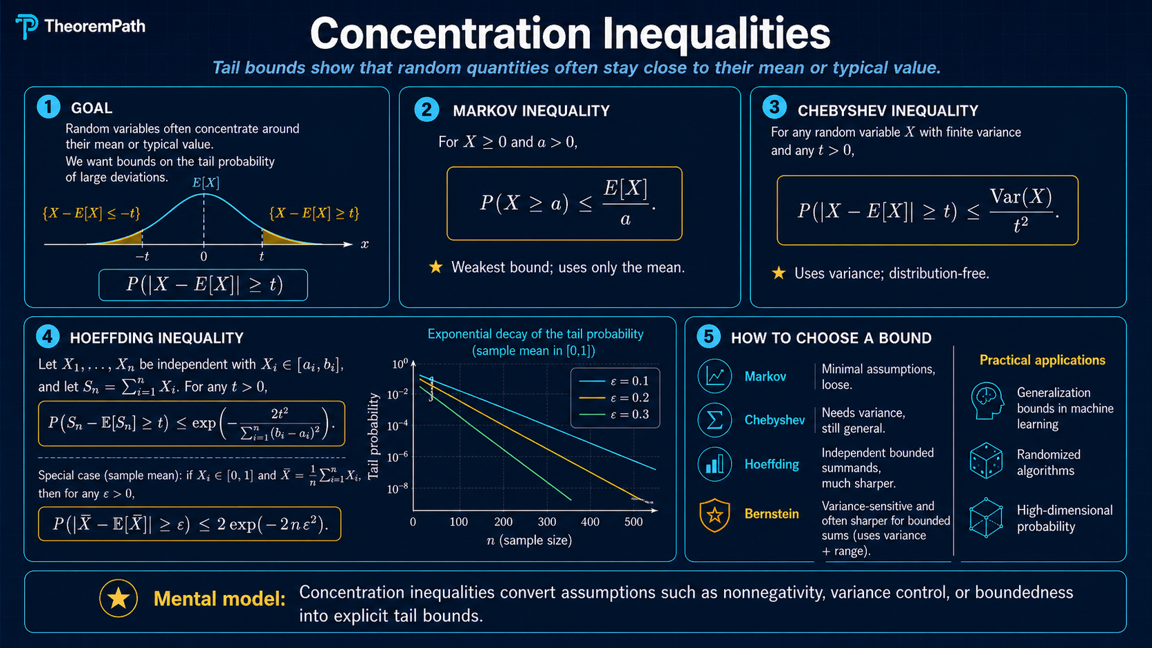
Bounds on how far random variables deviate from their expectations: Markov, Chebyshev, Hoeffding, and Bernstein. Used throughout generalization theory, bandits, and sample complexity.
Prerequisites
Why This Matters
Concentration inequalities are the backbone of classical uniform-convergence statistical learning theory. Most PAC-style sample complexity results and the core PAC-learning theorems ultimately rest on a statement of the form: "the empirical average is close to the true expectation with high probability." Modern generalization bounds (PAC-Bayes, algorithmic stability, information-theoretic bounds, and algorithm-dependent analyses) sometimes route through concentration only indirectly or replace boundedness assumptions with weaker moment / sub-Gaussian conditions, so the dependence is universal in spirit but not literal in form.
Hide overviewShow overview
When you see a bound like in ERM theory, the proof always invokes a concentration inequality. Without these tools, you cannot prove anything about learning from finite data.
These are the four inequalities you will use most often, in order of increasing power and increasing assumptions:
- Markov: requires only non-negativity
- Chebyshev: requires finite variance
- Hoeffding: requires bounded random variables
- Bernstein: requires bounded range and uses variance information
Mental Model
Think of concentration inequalities as answering one question: how likely is it that the sample average deviates from by more than ?
Each inequality trades assumptions for power:
- Markov/Chebyshev give polynomial tails (): slow decay.
- Hoeffding/Bernstein give exponential tails (): fast decay.
The exponential tail bounds are what make learning theory work. With polynomial tails, you need samples. With exponential tails, you need : the dependence on the confidence drops inside a logarithm.
Which Bound Should You Reach For?
This is the practical decision rule:
| What you know | Default bound | Tail shape | Why you reach for it |
|---|---|---|---|
| Only non-negativity | Markov | polynomial, | weakest possible structural assumption; useful as a first sanity bound |
| Finite variance but no bounded range | Chebyshev | polynomial, | works when variance is known but boundedness or MGF control is unavailable |
| Independent bounded summands | Hoeffding | exponential, roughly | clean default for finite-sample learning bounds and bounded losses |
| Independent bounded summands with genuinely small variance | Bernstein | Gaussian near the origin, then sub-exponential | variance-adaptive; much tighter when the loss is sparse or low-noise |
Stronger assumptions do not mean the resulting numeric bound is always smaller at every . The asymptotically stronger inequality can still be looser at modest sample sizes, which is why the worked example below compares Hoeffding and Chebyshev directly instead of repeating the slogan that "exponential beats polynomial."
Interactive: when Bernstein beats Hoeffding
Chebyshev, Hoeffding, and Bernstein all upper-bound the same tail probability. They do not agree on how much slack to leave. Plotted against the true binomial tail for with , the three bounds arrange themselves by the amount of variance information they use. Push toward and Bernstein splits away from Hoeffding because shrinks. Push to and the two exponential bounds nearly coincide.
Formal Setup and Notation
Let be independent random variables. We write for the sample mean and for its expectation (which equals when the are identically distributed).
We seek upper bounds on the tail probability:
or equivalently the one-sided tail .
Core Definitions
Tail Probability
The tail probability of a random variable at level is . Concentration inequalities provide upper bounds on tail probabilities, showing that is unlikely to deviate far from its mean. A bound is useful when it decays rapidly in .
Sub-Gaussian Behavior
A random variable exhibits sub-Gaussian behavior if and only if its tail probability decays like for some constant . Bounded random variables are sub-Gaussian (this is Hoeffding). The Gaussian decay rate is the "gold standard" for tail bounds. It means large deviations are exponentially unlikely.
Moment Generating Function
The moment generating function (MGF) of is . The MGF method — bounding the MGF and then optimizing over — is the standard technique for deriving exponential concentration inequalities. It is also called the Chernoff bounding method (Chernoff 1952); Wainwright (2019) uses this terminology. Cramér's theorem is a distinct, asymptotic result about the large-deviations rate function.
Main Theorems
Markov's Inequality
Statement
If , then for any :
Exact statement
LaTeX source for copy/export
\Pr[X \geq t] \leq \frac{\mathbb{E}[X]}{t}Intuition
If the average value of is small, then cannot be large too often. If , then can be at most 1% of the time; otherwise the average would be too high.
Proof Sketch
Indicator form.
Divide both sides by .
Integral (layer-cake) form. For , the tail formula gives
where the second inequality uses for every (the tail is nonincreasing). Divide by . This is the form used in Shalev-Shwartz and Ben-David, Understanding Machine Learning, Appendix B.
Why It Matters
Markov's inequality is the foundation that all other concentration inequalities build upon. Chebyshev applies Markov to . Hoeffding and Bernstein apply Markov to . It is the weakest bound but requires the fewest assumptions.
Failure Mode
The bound decays only as , polynomially. This is far too slow for most applications. If , Markov gives , independent of any variance or boundedness structure. For well-behaved distributions the true probability is astronomically smaller. Markov uses only ; it cannot see . Chebyshev is the first inequality that brings variance information into the picture. You almost always want Hoeffding or Bernstein when those assumptions hold.
Lemma B.1: Lower-tail bound for [0,1]-valued variables
Statement
If almost surely with , then for any :
Exact statement
LaTeX source for copy/export
\Pr[X > 1 - a] \geq \frac{\mu - (1 - a)}{a}Intuition
Markov bounds the upper tail of a nonnegative variable. The same idea applied to bounds the lower tail of . The lemma is most useful when is something like an accuracy in and you want a guarantee that is rarely far below its mean.
Proof Sketch
is nonnegative with . Markov's inequality gives . Take complements:
Why It Matters
This is the form of Markov used in the Shalev-Shwartz and Ben-David proof of agnostic PAC learnability of finite hypothesis classes. The argument needs a lower bound on the probability that the empirical risk is not too far below the true risk; Lemma B.1 supplies that bound from a one-sided expectation control.
Failure Mode
The bound is informative only when . If , the right-hand side is non-positive and the lemma reduces to the trivial bound . Like Markov itself, the bound uses only the mean and the boundedness range; it cannot see variance.
Chebyshev's Inequality
Statement
For any random variable with mean and finite variance , for any :
Exact statement
LaTeX source for copy/export
\Pr[|X - \mu| \geq t] \leq \frac{\sigma^2}{t^2}Intuition
Chebyshev uses variance information: if the spread of around its mean is small ( is small), then large deviations are unlikely. Applied to the sample mean, the variance decreases as , giving the familiar concentration.
Proof Sketch
Apply Markov's inequality to the nonnegative random variable . The square is monotone on nonnegative arguments, so if and only if :
Chebyshev is Markov applied to the squared deviation. This is the first place in the chain where the variance enters: Markov uses only , while Chebyshev squeezes one extra moment out of the same trick.
Why It Matters
Chebyshev gives the first quantitative form of the law of large numbers. For i.i.d. with mean and , the sample mean has variance
(by independence the cross-terms vanish). Combining this with Chebyshev gives . Equivalently, with probability , . Note the dependence, not .
Failure Mode
The decay is still polynomial. Chebyshev cannot give you the dependence needed for efficient learning. For bounded random variables, Hoeffding gives exponentially better tails. Chebyshev is most useful when you know the variance but nothing about higher moments or boundedness.
Lemma B.2: Chebyshev for the sample mean
Statement
Let be i.i.d. with and . For any , with probability at least :
Exact statement
LaTeX source for copy/export
\left|\frac{1}{m}\sum_{i=1}^m Z_i - \mu\right| \leq \sqrt{\frac{1}{\delta m}}Intuition
Solve Chebyshev for the deviation. Setting the failure probability and inverting for gives . With the normalization , the radius is .
Proof Sketch
Apply Chebyshev to with variance :
Set the right-hand side equal to and solve: . The complement event has probability .
Why It Matters
This is the explicit finite- form behind "the sample mean is close to ." It is the version of Chebyshev quoted as Lemma B.2 in Shalev-Shwartz and Ben-David, Understanding Machine Learning, Appendix B, where it sets up the polynomial sample-complexity baseline that exponential bounds later improve. The decay rate of the radius is : polynomial in , with a dependence on the confidence parameter.
Failure Mode
The rate is too slow for PAC-style sample complexity. For confidence and target accuracy , the lemma needs samples; Hoeffding under the same boundedness assumption needs roughly , an order of magnitude fewer. The dependence is the bottleneck.
From polynomial to exponential
Chebyshev gives a confidence interval of width — polynomial in , polynomial in . PAC learning needs better.
For accuracy at confidence , Lemma B.2 demands samples. The bottleneck is the dependence: halving the failure probability doubles the required .
Hoeffding's inequality, derived next, replaces this with exponential decay: for bounded random variables in ,
Inverting: . The same , now needs — about times fewer samples than Chebyshev. More importantly, halving adds only samples, a constant overhead instead of doubling.
The mechanism is the same Markov trick, applied to a different function. Markov uses only . Chebyshev applies Markov to and picks up the variance. The Chernoff/MGF method (used by Hoeffding and Bernstein) applies Markov to — the moment generating function — and picks up all polynomial moments at once. The exponential function dominates every polynomial; that is why exponential tails dominate polynomial tails.
| Inequality | Applied to | Tail decay in at fixed | dependence |
|---|---|---|---|
| Markov | none | ||
| Chebyshev | |||
| Hoeffding |
The polynomial-vs-exponential gap is what makes finite-sample learning theory work.
Sub-Gaussian Finite-Sum Tail Bound
Statement
Let be a finite independent family of centered sub-Gaussian random variables with MGF parameters . Then for any :
Exact statement
LaTeX source for copy/export
\Pr\!\left[\sum_{i \in I} Y_i \geq \epsilon\right] \leq \exp\!\left(-\frac{\epsilon^2}{2\sum_{i \in I} c_i}\right)Intuition
Sub-Gaussian MGF control behaves like variance under independent sums: the parameters add. Markov's inequality applied to then converts that MGF bound into an exponential tail bound.
Proof Sketch
Independence factors the MGF of the sum into a product of individual MGFs. The sub-Gaussian assumption bounds each factor by , so the product is bounded by . Apply Markov to the exponential transform and optimize .
Why It Matters
This is the exact formal bridge between concentration and finite-class learning bounds. Hoeffding for bounded losses first proves sub-Gaussian MGF control; the finite union bound then lifts the single-hypothesis tail bound to all hypotheses.
Failure Mode
The conclusion is a one-sided tail bound for a finite independent sum. It does not by itself prove the bounded-variable Hoeffding theorem or a uniform convergence theorem; those need additional assumptions and a union-bound step.
Hoeffding One-Sided Finite-Sum Bound
Statement
Let be a finite independent family of real random variables with almost surely. Then for :
Exact statement
LaTeX source for copy/export
\Pr\!\left[\sum_{i \in I} (X_i-\mathbb{E}X_i) \geq \epsilon\right] \leq \exp\!\left(-\frac{\epsilon^2}{2\sum_{i \in I} ((b_i-a_i)/2)^2}\right)Intuition
Bounded variables are sub-Gaussian after centering. Once each centered variable has sub-Gaussian MGF parameter , independence lets those parameters add across the finite sum.
Proof Sketch
Apply Hoeffding's lemma to each bounded variable to obtain sub-Gaussian MGF control for . Independence preserves that control under finite summation, and the sub-Gaussian finite-sum tail bound above converts the MGF statement into the displayed probability bound.
Why It Matters
This is the claim-facing bridge between bounded losses and finite-class uniform convergence. Setting gives the one-sided average Hoeffding form; applying the same argument to and union-bounding the two tails gives the common two-sided display.
Failure Mode
This statement covers the one-sided centered finite-sum bound. It does not by itself verify the two-sided display, the identical-bound special case, or a uniform convergence theorem; those need their own scoped claims or corollaries.
Hoeffding's Inequality
Statement
Let be independent random variables with almost surely. Then for any :
For the two-sided version:
Special case: If all (identically bounded):
Exact statement
LaTeX source for copy/export
\Pr\!\left[|\bar{X}_n - \mu| \geq t\right] \leq 2\exp\!\left(-\frac{2n^2t^2}{\sum_{i=1}^n (b_i-a_i)^2}\right)Intuition
Bounded random variables have sub-Gaussian tails. The width of the bounding interval controls the "effective variance" of each variable. The bound says: the probability of a deviation of size decays exponentially in , with the rate determined by how spread out the bounds are.
Proof Sketch
The proof uses the Chernoff/MGF method:
-
For any :
-
By independence:
-
Hoeffding's lemma: If , then
-
Combine and optimize over (set ).
Why It Matters
Hoeffding is the workhorse of learning theory. The ERM generalization bound for finite classes, the uniform convergence bound, and many other results use Hoeffding at their core. The exponential tail gives . The dependence is what makes high-confidence bounds feasible.
Failure Mode
Hoeffding uses only the range , not the actual variance. If the variance is much smaller than (e.g., a variable that is usually 0 but can be as large as 1), Hoeffding is loose. Bernstein fixes this by incorporating variance information.
Bernstein's Inequality
Statement
Let be independent with , , and almost surely. Then for any :
For the sample mean with i.i.d. variables ():
Exact statement
LaTeX source for copy/export
\Pr\!\left[\sum_{i=1}^n (X_i - \mu_i) \geq t\right] \leq \exp\!\left(-\frac{t^2/2}{\sum_{i=1}^n \sigma_i^2 + Mt/3}\right)Intuition
Bernstein interpolates between two regimes. For small deviations (), the term dominates the denominator and the bound looks like , a variance-dependent Gaussian tail. For large deviations (), the term dominates and the bound looks like , a sub-exponential tail. The variance term makes Bernstein much tighter than Hoeffding when the variance is small relative to the range.
Proof Sketch
Like Hoeffding, use the Chernoff method. The key improvement is a tighter bound on the MGF:
-
If and , then for .
-
This bound uses the variance instead of the crude range bound that Hoeffding uses.
-
Multiply over independent variables and optimize .
Why It Matters
Bernstein is the right inequality when you have variance information. In learning theory, this matters for sparse or low-noise settings. For example, if the loss is usually close to zero (low empirical risk, low variance), Bernstein gives much tighter bounds than Hoeffding, because Hoeffding only knows the loss is in while Bernstein knows the variance is small.
Failure Mode
Bernstein requires knowing (or bounding) the variance, which is not always available. If you only know the range , Hoeffding is simpler and sufficient. In practice, you can sometimes use an empirical estimate of the variance and apply Bernstein, but this introduces additional technical complications (you need a concentration bound on the variance estimate itself).
Proof Ideas and Templates Used
All four inequalities follow a common escalation pattern:
-
Markov's trick: the universal first step: convert a tail probability into an expectation bound via for any increasing .
-
Moment method: apply Markov to to get . Chebyshev is the case.
-
MGF/Chernoff method: apply Markov to for optimal . This is exponentially stronger because grows much faster than any polynomial. Both Hoeffding and Bernstein use this.
The key lemma in each exponential bound is controlling :
- Hoeffding's lemma bounds it using only boundedness:
- Bernstein's condition bounds it using variance:
Canonical Examples
Estimating a coin's bias with Hoeffding
Flip a coin times. Each flip with . The sample mean estimates . Hoeffding with gives:
For and : .
If we know (rare event), Bernstein with and gives roughly — about 19 times fewer samples. Bernstein exploits the small variance.
Comparing Markov, Chebyshev, and Hoeffding
Let be i.i.d. uniform on . We want .
Markov + Jensen (applied to , crude): first note that
So the standard deviation of is about .
Then
The first step is Markov on the non-negative random variable ; the second step is Jensen's inequality applied to , giving . Pure Markov on alone, without Jensen, would only give a bound in terms of and not in terms of the standard deviation.
Chebyshev: .
Hoeffding: . Hoeffding gives 0.27, which is worse than Chebyshev's 0.083.
Why: the Hoeffding exponent here is , so and the two-sided bound is . Chebyshev's is tighter because the exponent is simply not large enough for to beat at this . Hoeffding's exponential form dominates once is sufficiently larger than . For at the same , Hoeffding gives , beating Chebyshev's .
No single inequality is universally best at all sample sizes.
Hoeffding in learning theory: the finite-class ERM bound
The ERM generalization bound for :
For each fixed , the loss is a bounded random variable in . The empirical risk is the sample mean. Hoeffding gives:
Union bound over all :
This is how Hoeffding feeds directly into generalization bounds.
Common Confusions
Hoeffding requires bounded random variables, not just bounded variance
Hoeffding's inequality assumes almost surely. The random variables must be literally bounded. It does not apply to Gaussian random variables (which are unbounded), even though they have finite variance. For Gaussians, you use the exact sub-Gaussian tail , or you can use the sub-Gaussian framework that generalizes Hoeffding. If someone applies Hoeffding to an unbounded variable, the result is invalid.
Bernstein is better than Hoeffding when variance is small, not always
Bernstein's bound is , while Hoeffding gives . If (i.e., the variance is as large as it can be for the given range), Bernstein offers little or no improvement. Bernstein shines when . For example, when the random variable is usually near zero but has occasional large values. In the worst case over all distributions with given range, Hoeffding and Bernstein are comparable.
The two-sided Hoeffding bound is 2x the one-sided bound, not squared
A common error: writing . The factor of 2 comes from the union bound over the two tails: . Students sometimes confuse this with squaring the one-sided probability.
Summary
- Markov: . Weakest, needs only
- Chebyshev: . Uses variance, decay
- Hoeffding: . Exponential decay, needs boundedness
- Bernstein: like Hoeffding but uses variance . Tighter when
- Exponential tails give dependence in sample complexity; polynomial tails give
- The Chernoff/MGF method is the universal technique for deriving exponential bounds
- In learning theory, Hoeffding is the default; use Bernstein when you have variance information
Exercises
Problem
Using Hoeffding's inequality, how many fair coin flips do you need to estimate the probability of heads to within with probability at least 0.99?
Problem
Suppose are i.i.d. with , , and . Compare the sample sizes needed by Hoeffding and Bernstein to guarantee .
Problem
Prove Hoeffding's lemma: if and , then for all :
Related Comparisons
References
Reference note: this page is a pedagogical guide to the standard scalar concentration inequalities, not an exhaustive survey of martingale, matrix-valued, or geometric concentration.
Canonical:
- Hoeffding, W. (1963). "Probability Inequalities for Sums of Bounded Random Variables." Journal of the American Statistical Association.
- Boucheron, Lugosi, Massart, Concentration Inequalities: A Nonasymptotic Theory of Independence (2013), Chapters 2-3
- Shalev-Shwartz & Ben-David, Understanding Machine Learning, Appendix B
Current:
- Vershynin, High-Dimensional Probability (2018), Chapters 2-3
- Wainwright, High-Dimensional Statistics (2019), Chapter 2
- van Handel, Probability in High Dimension (2016), Chapters 1-3
Next Topics
Building on these basic inequalities:
- Sub-Gaussian random variables: the general framework unifying Hoeffding-type bounds
- Bernstein inequality: the variance-sensitive scalar bound
- Sub-exponential random variables: handling heavier tails (chi-squared, exponential distributions)
- McDiarmid's inequality: concentration for functions of independent variables, not just sums
- Contraction inequality: how Lipschitz transformations preserve concentration
Last reviewed: April 28, 2026
Claim evidence
Selected claims on this topic have machine-checked support.
Collapsed by default because this is audit material. Open it to see exact theorem names, claim scopes, and source roles.
Click to expand4
claim matches
0
dependency proofs
0
incomplete markers
Claim evidence
Selected claims on this topic have machine-checked support.
Collapsed by default because this is audit material. Open it to see exact theorem names, claim scopes, and source roles.
Click to expand4
claim matches
0
dependency proofs
0
incomplete markers
This is claim-level evidence, not a whole-page badge. The checked theorem must match the recorded claim scope. Supporting lemmas stay labeled as dependency proofs, not full claim matches.
Chebyshev inequality
Variance control gives a tail bound for deviations away from the mean.
Connects variance, moments, and concentration before stronger exponential bounds.
Formal record
- Checked theorem
- TheoremPath.Probability.Concentration.chebyshevInequalityVariance
- Claim scope
- real variance chebyshev inequality
- Proof scope
- exact mathlib wrapper for chebyshev
- Mathlib theorem
- ProbabilityTheory.meas_ge_le_variance_div_sq
Hoeffding one-sided finite-sum bound
A bounded independent finite sum has a one-sided exponential deviation bound.
A core theorem behind bounded-loss learning guarantees.
Formal record
- Checked theorem
- TheoremPath.Probability.Concentration.hoeffdingBoundedFiniteSumTail
- Claim scope
- finite centered sum bounded hoeffding one sided
- Proof scope
- exact mathlib wrapper for bounded hoeffding finite sum tail
- Mathlib theorem
- ProbabilityTheory.hasSubgaussianMGF_of_mem_Icc, ProbabilityTheory.iIndepFun.comp, ProbabilityTheory.HasSubgaussianMGF.measure_sum_ge_le_of_iIndepFun
Markov inequality
A nonnegative random variable with small expectation cannot be large very often.
First bridge from expectation control to a probability tail bound.
Formal record
- Checked theorem
- TheoremPath.Probability.Concentration.markovInequalityRealIntegrable
- Claim scope
- real integrable nonnegative markov inequality
- Proof scope
- exact mathlib wrapper for markov
- Mathlib theorem
- MeasureTheory.mul_meas_ge_le_integral_of_nonneg
Sub-Gaussian finite-sum tail bound
Independent sub-Gaussian variables have a finite-sum exponential tail bound.
Supports the concentration path toward finite-class generalization.
Formal record
- Checked theorem
- TheoremPath.Probability.Concentration.subGaussianFiniteSumTailBound
- Claim scope
- finite sum subgaussian tail bound
- Proof scope
- exact mathlib wrapper for subgaussian finite sum tail bound
- Mathlib theorem
- ProbabilityTheory.HasSubgaussianMGF.measure_sum_ge_le_of_iIndepFun
See the public evidence page for the display rules and representative Lean mapping examples.
Canonical graph
Required before and derived from this topic
These links come from prerequisite edges in the curriculum graph. Editorial suggestions are shown here only when the target page also cites this page as a prerequisite.
Required prerequisites
12- Common Inequalitieslayer 0A · tier 1
- Common Probability Distributionslayer 0A · tier 1
- Expectation, Variance, Covariance, and Momentslayer 0A · tier 1
- Sets, Functions, and Relationslayer 0A · tier 1
- Central Limit Theoremlayer 0B · tier 1
Derived topics
24- Chernoff Boundslayer 1 · tier 1
- Hoeffding's Lemmalayer 1 · tier 1
- PAC Learning Frameworklayer 1 · tier 1
- Bennett's Inequalitylayer 2 · tier 1
- Bernstein Inequalitylayer 2 · tier 1
+19 more on the derived-topics page.
Graph-backed continuations