PAC Learning Framework

Why This Matters

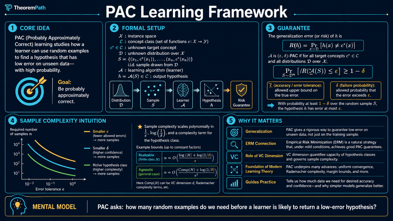
The PAC (Probably Approximately Correct) framework, introduced by Leslie Valiant in 1984, is the mathematical foundation for answering the most basic question in machine learning: when is it possible to learn from data?

Hide overviewShow overview

Before PAC theory, machine learning was a collection of algorithms without a unifying theory of learnability. PAC provides the definitions and theorems that tell you whether a learning problem is solvable in principle, and how many samples you need.

Every generalization bound you encounter, from ERM to VC dimension to Rademacher complexity, is ultimately answering a question that PAC theory formalized. The sample complexity bounds page covers the quantitative details.

Mental Model

Think of a learner as a detective. The detective wants to identify an unknown rule (the target concept) but can only observe examples. PAC theory asks: how many examples does the detective need to be probably ($1 - \delta$) approximately ($\epsilon$) correct about the rule?

The "probably" accounts for the randomness of the training sample. you might get an unlucky draw. The "approximately" accounts for the fact that you do not need to identify the rule exactly; getting close is enough.

Formal Setup and Notation

Let $\mathcal{X}$ be an instance space (e.g., $\{0,1\}^n$). A concept is a function $c: \mathcal{X} \to \{0, 1\}$. A concept class $\mathcal{C}$ is a collection of concepts.

There is an unknown distribution $\mathcal{D}$ over $\mathcal{X}$ and an unknown target concept $c^* \in \mathcal{C}$.

The learner receives a training sample

$S = \{(x_1, c^*(x_1)), \ldots, (x_n, c^*(x_n))\}$

where each $x_i \sim \mathcal{D}$ independently.

The learner outputs a hypothesis $h: \mathcal{X} \to \{0, 1\}$.

Definition

Generalization Error

The generalization error (or risk) of a hypothesis $h$ with respect to target $c^*$ and distribution $\mathcal{D}$ is:

$R(h) = \Pr_{x \sim \mathcal{D}}[h(x) \neq c^*(x)]$

This is the probability that $h$ disagrees with $c^*$ on a random example.

Core Definitions

Definition

PAC Learnability (Realizable Case)$PAC$

A concept class $\mathcal{C}$ is PAC-learnable if and only if there exists an algorithm $\mathcal{A}$ and a function $n_{\mathcal{C}}: (0,1)^2 \to \mathbb{N}$ such that for every target concept $c^* \in \mathcal{C}$, every distribution $\mathcal{D}$ over $\mathcal{X}$, every accuracy parameter $\epsilon \in (0, 1)$, and every confidence parameter $\delta \in (0, 1)$:

when $\mathcal{A}$ is given a sample $S$ of size $n \geq n_{\mathcal{C}}(\epsilon, \delta)$ drawn i.i.d. from $\mathcal{D}$ and labeled by $c^*$, it outputs $h$ satisfying:

$\Pr_S[R(h) \leq \epsilon] \geq 1 - \delta$

The class is polynomial-sample PAC-learnable if $n_{\mathcal{C}}(\epsilon, \delta)$ is polynomial in $1/\epsilon$ and $1/\delta$. It is efficiently PAC-learnable (also called polynomial-time PAC-learnable) if, in addition, $\mathcal{A}$ runs in time polynomial in $1/\epsilon$, $1/\delta$, and $\text{size}(c^*)$. This follows the standard usage in computational learning theory (Valiant 1984, Kearns and Vazirani 1994), where "efficient" always refers to time, not sample, complexity.

The key features of this definition:

1. For all distributions. The learner must work regardless of $\mathcal{D}$
2. For all target concepts. The learner must work for any $c^* \in \mathcal{C}$
3. Probably: the guarantee holds with probability $\geq 1 - \delta$
4. Approximately: the error is at most $\epsilon$, not necessarily zero

Definition

Sample Complexity

The sample complexity $n_{\mathcal{C}}(\epsilon, \delta)$ is the minimum number of training examples needed to achieve error $\leq \epsilon$ with confidence $\geq 1 - \delta$. This is the fundamental quantity that PAC theory characterizes.

Realizable vs. Agnostic PAC

Definition

Realizable Setting

In the realizable setting, we assume $c^* \in \mathcal{C}$. The target concept is in our hypothesis class. The learner can achieve zero training error. The question is whether zero training error implies low test error.

Definition

Agnostic PAC Learning

In the agnostic setting, we make no assumption about the target. Labels may be generated by any joint distribution over $\mathcal{X} \times \{0,1\}$. The goal is to compete with the best hypothesis in $\mathcal{C}$:

$\Pr_S\!\left[R(h) \leq \min_{h' \in \mathcal{C}} R(h') + \epsilon\right] \geq 1 - \delta$

This is harder because even the best hypothesis in $\mathcal{C}$ may have nonzero error (the approximation error). Agnostic PAC learning requires more samples.

The agnostic setting is more realistic: in practice, you never know if the true relationship is exactly representable by your model class.

What breaks when realizability is dropped. Under realizability, the single-hypothesis tail used $\Pr[h \text{ consistent}] \leq (1 - \epsilon)^n$, which is a Bernoulli-on-clean-flips event: each independent example has probability $\geq \epsilon$ of exposing a bad $h$. In the agnostic setting there is no $h$ with zero population error to anchor against, so the relevant question becomes "how close is $\hat{R}_n(h)$ to $R(h)$ uniformly?" That is a concentration question, answered by Hoeffding: for a single bounded $h$, $\Pr[|\hat{R}_n(h) - R(h)| > \epsilon] \leq 2 e^{-2n\epsilon^2}$. The exponent flips from $-n\epsilon$ to $-n\epsilon^2$, and inverting it gives $n = O(\log(M/\delta)/\epsilon^2)$ instead of $O(\log(M/\delta)/\epsilon)$. The square is the unavoidable cost of estimating an unknown mean rather than detecting a single bad consistent hypothesis. See the realizable vs. agnostic comparison for the side-by-side derivation.

Main Theorems

Theorem

PAC Bound for Finite Hypothesis Classes

Statement

Let $\mathcal{C}$ be a finite concept class with $|\mathcal{C}| = M$. In the realizable setting, the ERM algorithm (which outputs any $h \in \mathcal{C}$ consistent with the training data) satisfies: for any $\epsilon, \delta > 0$, if the sample size satisfies:

$n \geq \frac{1}{\epsilon}\left(\log M + \log \frac{1}{\delta}\right)$

then with probability $\geq 1 - \delta$, the output $h$ has $R(h) \leq \epsilon$.

Intuition

Each "bad" hypothesis (one with error $> \epsilon$) has probability at most $(1 - \epsilon)^n \leq e^{-n\epsilon}$ of being consistent with all $n$ training examples. There are at most $M$ bad hypotheses. By a union bound, the probability that any bad hypothesis survives is at most $M e^{-n\epsilon}$. Setting this $\leq \delta$ and solving for $n$ gives the bound.

Proof Sketch

The proof is a clean three-step union-bound argument. We give every step explicitly because this template recurs throughout statistical learning theory.

Step 1: Single-hypothesis tail. Fix one hypothesis $h \in \mathcal{C}$ with $R(h) > \epsilon$. Call $h$ bad. For one random example $(x_i, c^*(x_i))$ with $x_i \sim \mathcal{D}$, the probability that $h(x_i) = c^*(x_i)$ is at most $1 - \epsilon$ (because $h$ disagrees with $c^*$ on at least an $\epsilon$ fraction of $\mathcal{D}$). Independence across the $n$ training points gives:

$\Pr_S[h \text{ consistent with } S] = \prod_{i=1}^n \Pr[h(x_i) = c^*(x_i)] \leq (1 - \epsilon)^n$

The convexity inequality $1 - x \leq e^{-x}$ for $x \geq 0$ (the tangent line to $e^{-x}$ at $x = 0$) tightens this to:

$\Pr_S[h \text{ consistent with } S] \leq (1 - \epsilon)^n \leq e^{-n\epsilon}$

Step 2: Union bound over the bad set. Let $\mathcal{C}_{\text{bad}} = \{h \in \mathcal{C} : R(h) > \epsilon\}$, with $|\mathcal{C}_{\text{bad}}| \leq |\mathcal{C}| = M$. ERM fails when some bad hypothesis is consistent with $S$ (because then ERM may return it). The union bound gives:

$\Pr_S\!\left[\exists h \in \mathcal{C}_{\text{bad}} : h \text{ consistent with } S\right] \leq \sum_{h \in \mathcal{C}_{\text{bad}}} e^{-n\epsilon} \leq M e^{-n\epsilon}$

The factor of $M$ is the price for searching over the whole class. Note it enters additively across hypotheses, which is what allows the logarithm to absorb it in the next step.

Step 3: Solve for $n$. We want the failure probability $\leq \delta$:

$M e^{-n\epsilon} \leq \delta \iff e^{-n\epsilon} \leq \frac{\delta}{M} \iff n\epsilon \geq \log\frac{M}{\delta}$

Rearranging gives the sample complexity:

$n \geq \frac{1}{\epsilon}\left(\log M + \log\frac{1}{\delta}\right)$

The logarithmic dependence on $M$ is the key. A class with $2^d$ hypotheses needs only $O(d/\epsilon)$ samples, not $O(2^d/\epsilon)$. This is what makes ERM tractable even for combinatorially large finite classes. For infinite classes, $\log M = \infty$ and this argument fails; VC theory replaces $\log M$ with the VC dimension $d_{\text{VC}}$ via symmetrization and the Sauer-Shelah lemma.

Why It Matters

This is the simplest PAC bound and the template for all subsequent results. The sample complexity is $O(\frac{1}{\epsilon}\log M)$. logarithmic in the size of the hypothesis class. This logarithmic dependence is what makes learning from finite classes tractable even when $M$ is exponentially large.

Failure Mode

This bound requires the realizable assumption ($c^* \in \mathcal{C}$). In the agnostic case, the rate changes from $O(1/\epsilon)$ to $O(1/\epsilon^2)$. The square is the cost of not knowing the target is in your class.

report a correction →

Theorem

Fundamental Theorem of PAC Learning

Statement

For binary classification with 0-1 loss, the following are equivalent:

1. $\mathcal{C}$ has finite VC dimension
2. $\mathcal{C}$ is agnostic PAC-learnable
3. $\mathcal{C}$ is PAC-learnable (realizable case)
4. ERM over $\mathcal{C}$ is a successful agnostic PAC learner

Moreover, the sample complexity of agnostic PAC learning is:

$n_{\text{agnostic}} = \Theta\!\left(\frac{d_{\text{VC}} + \log(1/\delta)}{\epsilon^2}\right)$

and in the realizable case (where some $c^* \in \mathcal{C}$ has zero risk):

$n_{\text{realizable}} = O\!\left(\frac{d_{\text{VC}} \log(1/\epsilon) + \log(1/\delta)}{\epsilon}\right)$

where $d_{\text{VC}}$ is the VC dimension of $\mathcal{C}$. The realizable case scales as $1/\epsilon$ rather than $1/\epsilon^2$, the same quadratic- versus-linear gap that appeared in the finite-class bound, now expressed in $d_{\text{VC}}$ instead of $\log|\mathcal{C}|$. The $\log(1/\epsilon)$ factor in the realizable upper bound is removable for proper realizable learners (Hanneke 2016, JMLR), giving the optimal $\Theta((d_{\text{VC}} + \log(1/\delta))/\epsilon)$ rate.

Intuition

The VC dimension is the exact measure of hypothesis class complexity that determines learnability. A class is learnable if and only if it cannot shatter arbitrarily large sets of points. The VC dimension replaces the crude $\log M$ of the finite case with a geometric measure of complexity that works for infinite classes.

Why It Matters

This is the most important theorem in statistical learning theory. It completely characterizes PAC learnability: finite VC dimension is both necessary and sufficient. Every other complexity measure (Rademacher complexity, covering numbers, fat-shattering dimension) can be related back to this fundamental characterization.

Failure Mode

This theorem applies only to binary classification with 0-1 loss. For regression, multi-class classification, or other loss functions, the characterization is more complex and involves different complexity measures.

report a correction →

Proof Ideas and Templates Used

The proofs in PAC theory repeatedly use two techniques:

1. Union bound + pointwise concentration: Bound the probability that a single hypothesis is misleading (pointwise), then take a union bound over all hypotheses. This works for finite classes.

2. Symmetrization + growth function: For infinite classes, the union bound over hypotheses is replaced by a union bound over behaviors of hypotheses on a ghost sample. The number of distinct behaviors is bounded by the growth function $\Pi_{\mathcal{C}}(n)$, which is polynomial in $n$ when the VC dimension is finite (Sauer's lemma).

Canonical Examples

Example

Learning conjunctions

The class of conjunctions over $n$ Boolean variables contains $3^n$ hypotheses (each variable can appear positive, negative, or absent). The PAC bound gives sample complexity $O(\frac{n}{\epsilon}\log 3) = O(\frac{n}{\epsilon})$. There is also a simple polynomial-time algorithm: start with all literals and remove any literal falsified by a positive example.

Example

Learning intervals on the real line

The class of intervals $[a, b] \subset \mathbb{R}$ has VC dimension 2. By the fundamental theorem, the sample complexity for agnostic PAC learning is $O(1/\epsilon^2)$, independent of the number of possible intervals (which is uncountably infinite).

Worked Example: Numeric Walkthrough

Take a concrete tier of accuracy targets and compare what the realizable finite-class bound, the VC realizable bound, and the agnostic VC bound actually demand. Fix $d_{\text{VC}} = 10$ (a small parametric class such as a 10-dimensional halfspace family with margin), and set $\delta = 0.05$ throughout.

Realizable finite-class bound (from $n \ge \frac{1}{\epsilon}(\log M + \log(1/\delta))$, with $M = 2^{d_{\text{VC}}} = 1024$):

The bound scales as $1/\epsilon$. Halving $\epsilon$ doubles the sample requirement.

Agnostic VC bound (from $n = \Theta((d_{\text{VC}} + \log(1/\delta))/\epsilon^2)$, dropping $\Theta$ constants):

The agnostic bound scales as $1/\epsilon^2$. Halving $\epsilon$ quadruples the sample requirement. At $\epsilon = 0.01$, the agnostic case demands $\sim 130\times$ more data than the realizable finite-class bound — the quadratic price of not knowing whether the target is in your class. This factor blows up further as $\epsilon$ shrinks, which is why agnostic guarantees at very small error tolerances are expensive in practice.

The ratio of agnostic-to-realizable sample complexity is $\Theta(1/\epsilon)$ — a ratio that grows as you demand smaller error. At $\epsilon = 0.001$, the agnostic bound is already $\sim 1000\times$ larger than the realizable bound. This gap is the formal content of the agnostic-vs-realizable comparison.

Lower Bounds: The Bound Is Tight

The upper bounds above are not loose. For binary classification, the agnostic VC sample complexity is tight up to logarithmic factors: there exist matching lower bounds.

Theorem

Sample-Complexity Lower Bound for VC Classes

Statement

For every PAC learning algorithm $\mathcal{A}$ and every concept class $\mathcal{C}$ with $d_{\text{VC}}(\mathcal{C}) = d$, there exist distributions and target concepts on which $\mathcal{A}$ requires at least

$$n \ge c \cdot \frac{d + \log(1/\delta)}{\epsilon^2}$$

samples to achieve $\Pr[R(h) \le \epsilon] \ge 1 - \delta$ in the agnostic setting, for an absolute constant $c > 0$.

Intuition

The lower bound is constructed by exhibiting a hard distribution: pick $d$ shattered points and randomize their labels. Any algorithm with too few samples must miss at least one of the $2^d$ possible labellings, and for that labelling its hypothesis is forced to error $\Theta(\epsilon)$. The $1/\epsilon^2$ rate emerges from the variance of empirical-risk estimates on the hard distribution; it cannot be improved without distribution-specific assumptions.

Why It Matters

This says the agnostic PAC sample complexity is tight up to constants and logarithmic factors. You cannot beat $1/\epsilon^2$ in the worst case, no matter what algorithm you design. Any improvement must come from distribution-specific structure (margin, low noise, smoothness) — the content of fast-rate generalization theory.

Failure Mode

The lower bound requires an adversarial distribution. Real data has structure (margin, smoothness, low noise) that allows faster rates. The $1/\epsilon^2$ floor is for the worst-case PAC framework, not for any specific distribution.

report a correction →

The realizable PAC bound has an analogous matching lower bound at $n = \Omega(d/\epsilon)$, also up to log factors. So the entire PAC framework is essentially complete: VC dimension determines sample complexity, and the bounds are tight.

Connection to Uniform Convergence

The PAC framework and the uniform convergence framework are two sides of the same coin. PAC asks: how many samples does a learner need? Uniform convergence asks: how fast does the empirical risk converge to the true risk uniformly over the hypothesis class? The two are equivalent for binary classification with 0-1 loss.

The bridge: a class is agnostic PAC-learnable if and only if its loss class is a Glivenko-Cantelli class — exactly the classes for which $\sup_h |R_n(h) - R(h)| \to 0$ uniformly. ERM is a successful agnostic PAC learner because uniform convergence ensures the empirical-risk minimizer is close to the population-risk minimizer.

For finite classes: uniform convergence follows from a union bound and Hoeffding's inequality. For infinite classes with finite VC dimension: uniform convergence follows from symmetrization plus the Sauer-Shelah polynomial growth bound on the number of distinct hypothesis behaviors on $n$ points. Both routes yield the same $O(1/\epsilon^2)$ agnostic rate.

Common Confusions

Watch Out

PAC learnability is distribution-free

The PAC guarantee must hold for every distribution $\mathcal{D}$. This is a very strong requirement. It means the sample complexity bounds are worst-case over distributions. For specific, well-behaved distributions, you might need far fewer samples. This is both the strength (universality) and weakness (conservatism) of PAC theory.

Watch Out

Efficient learnability requires polynomial time

PAC learnability as defined above only requires polynomial sample complexity. It says nothing about computational efficiency. A class can be PAC-learnable (finite VC dimension) but not efficiently PAC-learnable (finding the ERM hypothesis is NP-hard). For example, learning intersections of halfspaces is PAC-learnable but believed to be computationally hard.

Watch Out

The realizable assumption is very strong

Assuming $c^* \in \mathcal{C}$ means you know the true concept is representable by your hypothesis class. In practice, this is almost never true: real models always face some degree of overfitting. The agnostic setting is more realistic but requires $O(1/\epsilon^2)$ samples instead of $O(1/\epsilon)$. The quadratic cost of agnosticism is a fundamental price you pay for not knowing the true model.

Summary

• PAC = Probably ($1-\delta$) Approximately ($\epsilon$) Correct
• Sample complexity for finite class (realizable): $n = O(\frac{1}{\epsilon}\log|\mathcal{C}|)$
• Sample complexity for finite VC dimension (agnostic): $n = O(\frac{d_{\text{VC}}}{\epsilon^2})$
• The fundamental theorem: finite VC dimension is equivalent to PAC learnability for binary classification
• PAC is distribution-free: bounds hold for the worst-case distribution
• Computational complexity is a separate question from sample complexity

Exercises

ExerciseCore

Problem

A concept class $\mathcal{C}$ has 256 concepts. In the realizable setting, how many samples do you need to guarantee that with probability at least $0.9$, the ERM hypothesis has error at most $0.05$?

Hint

Reveal Solution

ExerciseCore

Problem

Explain in one sentence why the sample complexity for the agnostic case is $O(1/\epsilon^2)$ while the realizable case is $O(1/\epsilon)$.

Hint

Reveal Solution

ExerciseAdvanced

Problem

The class of all Boolean functions on $n$ bits has $2^{2^n}$ concepts. What is the PAC sample complexity in the realizable case? Is this class efficiently PAC-learnable?

Hint

Reveal Solution

Related Comparisons

• PAC Learning vs. Agnostic PAC Learning

References

Canonical:

• Valiant, "A Theory of the Learnable," Communications of the ACM (1984)
• Shalev-Shwartz & Ben-David, Understanding Machine Learning, Chapters 2-6
• Kearns & Vazirani, An Introduction to Computational Learning Theory (1994), Chapters 1-3

Current:

• Mohri, Rostamizadeh, Talwalkar, Foundations of Machine Learning (2018), Chapter 2
• Wainwright, High-Dimensional Statistics (2019), Chapters 4-6
• Bartlett & Mendelson, "Rademacher and Gaussian Complexities: Risk Bounds and Structural Results," JMLR 3 (2002), 463-482. The Rademacher route to PAC bounds; often tighter than the VC route and the standard reference for data-dependent generalization analysis. jmlr.org
• Hopkins, Kane, Lovett, Mahajan, "Realizable Learning is All You Need," COLT (2022), arXiv:2111.04746 — proves that for any concept class, agnostic learnability is equivalent to realizable learnability up to a polynomial sample-complexity blowup
• Brukhim, Carmon, Dinur, Moran, Yehudayoff, "A Characterization of Multiclass Learnability," FOCS (2022), arXiv:2203.01550 — closes the multiclass case with the DS dimension, settling a 30-year open problem about which multiclass classes are PAC-learnable

Next Topics

The natural next steps from PAC learning:

• Empirical risk minimization: the algorithmic principle that implements PAC learning
• VC dimension: the complexity measure that characterizes PAC learnability