Foundations
Differentiation in Rⁿ
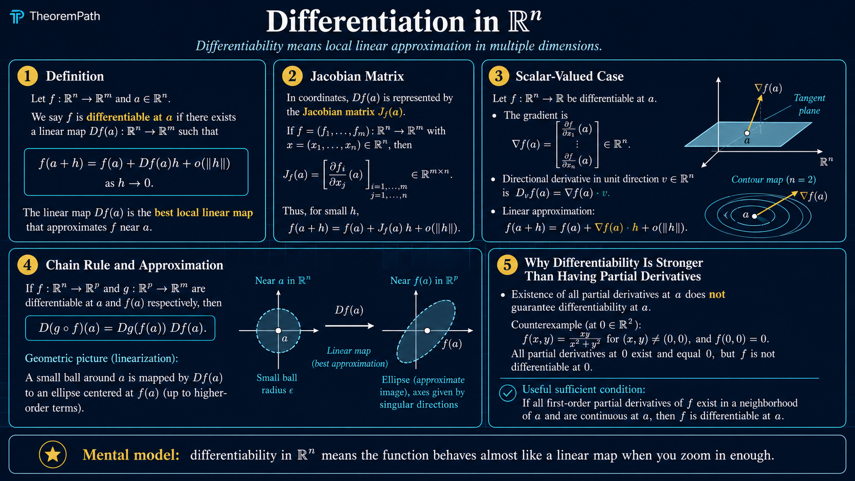
Partial derivatives, directional derivatives, gradients, total derivatives, and the multivariable chain rule. The point is not notation: differentiability means one linear map predicts all small directions.
Why This Matters
Machine learning optimization is built on one sentence:
Hide overviewShow overview
Near the current parameters, replace the loss by a linear or quadratic approximation, then choose a step.
That sentence only makes sense if you understand differentiation in . Gradients tell SGD and Adam which way the loss changes. Jacobians compose through neural-network layers. Hessians explain curvature, Newton steps, conditioning, and why a learning rate can explode.
The trap is thinking that multivariable differentiation is just "take partial derivatives." It is stricter than that. The real object is the total derivative: one linear map that predicts the function for every small direction at once.
The Local Linear Model
For , differentiability at means there is a linear map such that
The remainder must be small compared with the step length . This is the multivariable version of a tangent line, but now the tangent object is a linear map.
Coordinate Derivatives
Partial Derivative
For , the partial derivative with respect to coordinate at is
It measures change when only the th coordinate moves.
Partial derivatives are coordinate probes. They are useful, but they do not by themselves prove the function has a good local linear approximation in every direction.
Directional Derivative
For a unit vector , the directional derivative is
It measures the rate of change along the line through in direction .
Directional derivatives probe more directions than partial derivatives, but even all directional derivatives existing is not the same thing as differentiability. Differentiability requires those directional rates to come from one linear map.
Gradient And Total Derivative
Gradient
For a scalar-valued function , the gradient is the column vector
When is differentiable, .
The gradient is the vector representation of the total derivative for scalar outputs. The total derivative itself is a linear functional, often written as a row vector. This row-versus-column distinction matters when multiplying Jacobians in the chain rule.
Jacobian Matrix
For , the total derivative is represented by the by Jacobian matrix
The Jacobian maps input perturbations to first-order output perturbations.
Steepest Direction
Gradient As Steepest Ascent Direction
Statement
If , then among all unit vectors , the directional derivative is maximized by , and the maximum value is . The minimum is achieved in the negative-gradient direction with value .
If , the expression is undefined; in this case every directional derivative satisfies , every unit vector is simultaneously a maximizer and minimizer, and there is no first-order steepest direction. Determining whether is a min, max, or saddle requires second-order information (the Hessian).
Intuition
The dot product is largest when two vectors point in the same direction. The gradient points uphill fastest; the negative gradient points downhill fastest for an infinitesimal Euclidean step.
Proof Sketch
By Cauchy-Schwarz, . Equality holds exactly when is a positive scalar multiple of . The minimum follows by using the opposite direction.
Why It Matters
This is the mathematical reason gradient descent, SGD, and Adam use as their primary signal.
Failure Mode
This is an infinitesimal claim. A finite step can overshoot because curvature enters through higher-order terms. That is why line search, learning-rate schedules, and second-order methods exist.
When Partials Are Enough
Continuous Partial Derivatives Imply Differentiability
Statement
If all first partial derivatives of exist in a neighborhood of and are continuous at , then is differentiable at .
Intuition
Continuity of the partial derivatives prevents coordinate-wise rates from changing wildly as you approach the point from different directions. The coordinate probes assemble into one stable linear approximation.
Proof Sketch
Write as a telescoping sum that changes one coordinate at a time. Apply the one-variable mean value theorem to each coordinate change. Continuity of the partial derivatives turns each coefficient into the corresponding partial derivative at plus a small error. The sum becomes .
Why It Matters
Most smooth ML losses satisfy this condition away from nonsmooth activations or constraints, so computing the Jacobian from partial derivatives is usually legitimate.
Chain Rule
Multivariable Chain Rule
Statement
If is differentiable at and is differentiable at , then is differentiable at and
Intuition
Each differentiable map is locally linear. Composing functions locally composes their linear approximations, so the derivative of the composition is matrix multiplication.
Proof Sketch
Use . Then apply the differentiability of at to the perturbation . Linearity of produces plus a remainder smaller than .
Why It Matters
Backpropagation is the chain rule on a computational graph. A network is a composition of layers; reverse-mode automatic differentiation multiplies local derivatives in the direction that is efficient for scalar losses.
Failure Mode
Nonsmooth points such as ReLU at zero break classical differentiability. Optimizers still work by using subgradients or implementation conventions, but theorem assumptions should not be silently ignored.
ML Translation Table
| Math object | ML interpretation | What to check |
|---|---|---|
| parameters, features, or activations | which variable is being differentiated | |
| loss, layer map, score, or metric | scalar or vector output | |
| first-order signal for update direction | norm, scale, noise, clipping | |
| / Jacobian | local sensitivity of outputs to inputs | shape, conditioning, chain rule order |
| / Hessian | curvature of the scalar loss | positive definite, indefinite, ill-conditioned |
| ignored higher-order error | when finite steps make the linear model invalid |
Common Confusions
Partial derivatives existing is not enough
There are functions with all partial derivatives at a point that are not continuous there, and therefore not differentiable. Partial derivatives are coordinate checks; differentiability is an all-directions linear approximation.
The gradient is not the derivative for vector outputs
For , the gradient represents the derivative. For , the derivative is a Jacobian matrix, not a single gradient vector.
Steepest descent depends on the norm
The Euclidean gradient is steepest for Euclidean step size. If you change the geometry, the steepest direction changes. Natural gradient and preconditioned methods exploit exactly this fact.
Backprop is not magic
Backpropagation is not a separate calculus. It is the multivariable chain rule organized efficiently so that scalar loss gradients are computed without forming every full Jacobian.
Q&A For Mastery
Why does differentiability require an open neighborhood? You need to approach the point from many directions. On a boundary or constrained set, ordinary derivatives may need to be replaced by restricted, one-sided, or manifold derivatives.
What should I remember for neural networks? Each layer has a local derivative. Backprop multiplies those local derivatives in reverse order to get gradients with respect to parameters.
Why do gradients vanish or explode? Long products of Jacobians can shrink or amplify vectors. This is the calculus reason recurrent nets and deep networks need normalization, residual connections, initialization care, and gating.
What is the practical shape check? If , then is by . Multiplying should produce a vector in .
What To Remember
- Differentiability means one linear map approximates all small directions.
- Partial derivatives are coordinate probes, not the whole story.
- For scalar outputs, .
- The negative gradient is the steepest infinitesimal descent direction in Euclidean geometry.
- The chain rule is matrix multiplication of local linear maps.
- Backpropagation is the chain rule arranged for computational efficiency.
Exercises
Problem
Let . Compute and the directional derivative in direction .
Problem
Suppose is differentiable at . Prove that if , then every directional derivative at equals zero.
Problem
Explain why ReLU networks can be trained with gradient methods even though ReLU is not differentiable at zero.
References
Canonical:
- Rudin, Principles of Mathematical Analysis, 3rd ed., Chapter 9.
- Spivak, Calculus on Manifolds, Chapter 2.
- Apostol, Mathematical Analysis, 2nd ed., Chapter 12.
ML-facing:
- Deisenroth, Faisal, and Ong, Mathematics for Machine Learning, Chapter 5.
- Goodfellow, Bengio, and Courville, Deep Learning, Chapter 4.
- Boyd and Vandenberghe, Convex Optimization, Appendix A.4.
Next Topics
- The Jacobian matrix: the full derivative matrix for vector-valued maps.
- Vector calculus chain rule: deeper shape discipline for composition.
- Automatic differentiation: how software computes gradients efficiently.
- The Hessian matrix: second-order local models and curvature.
Last reviewed: April 26, 2026
Canonical graph
Required before and derived from this topic
These links come from prerequisite edges in the curriculum graph. Editorial suggestions are shown here only when the target page also cites this page as a prerequisite.
Required prerequisites
3- Continuity in Rⁿlayer 0A · tier 1
- Sets, Functions, and Relationslayer 0A · tier 1
- Vectors, Matrices, and Linear Mapslayer 0A · tier 1
Derived topics
11- Taylor Expansionlayer 0A · tier 1
- The Hessian Matrixlayer 0A · tier 1
- The Jacobian Matrixlayer 0A · tier 1
- Vector Calculus Chain Rulelayer 0A · tier 1
- Maximum Likelihood Estimation: Theory, Information Identity, and Asymptotic Efficiencylayer 0B · tier 1
+6 more on the derived-topics page.
Graph-backed continuations