Riemannian Optimization and Manifold Constraints

Why This Matters

Standard gradient descent assumes parameters live in flat Euclidean space $\mathbb{R}^d$. But many ML problems have constraints that define curved spaces: weight matrices that must stay orthogonal, covariance matrices that must stay positive definite, probability distributions that must stay on the simplex, or embeddings that must stay on a sphere.

Hide overviewShow overview

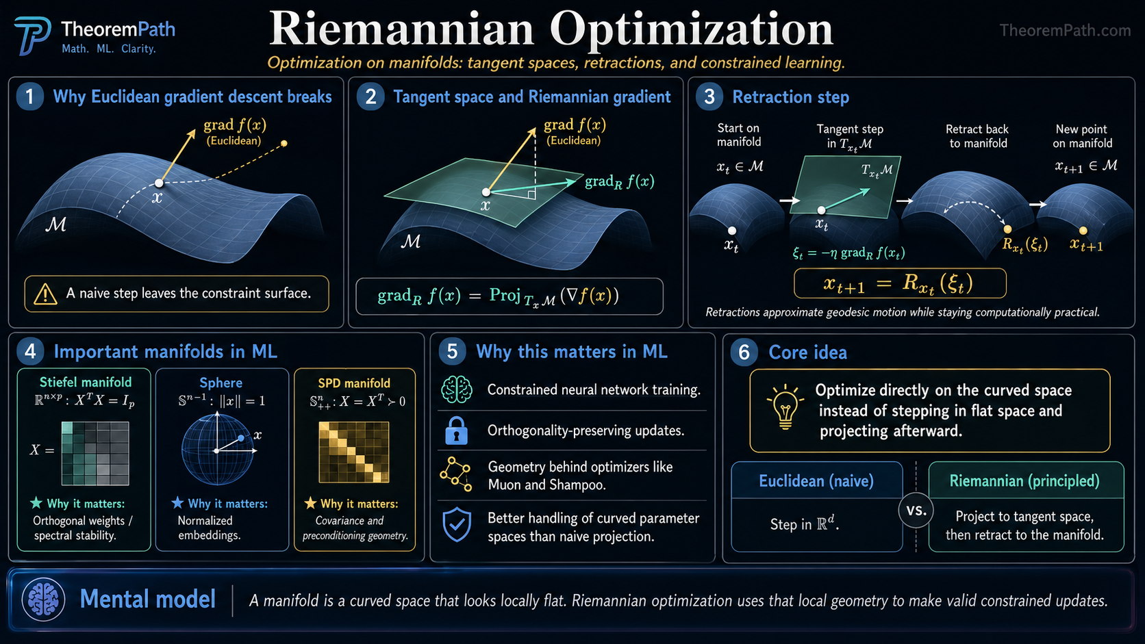
If you just project back to the constraint set after each gradient step, you waste computation and can get poor convergence. Riemannian optimization does better: it works directly on the curved surface (manifold), computing gradients that are tangent to the surface and taking steps that stay on it.

This is not esoteric geometry. The Muon optimizer uses Newton-Schulz iteration to approximate projection onto the Stiefel manifold. Shampoo preconditions gradients using the space of symmetric positive definite matrices. Understanding the manifold geometry explains why these optimizers work and where they fail.

Core Concepts

Definition

Smooth Manifold$\mathcal{M}$

A smooth manifold $\mathcal{M}$ is a space that locally looks like $\mathbb{R}^d$ but may be globally curved. Each point $p \in \mathcal{M}$ has a tangent space $T_p\mathcal{M}$, a vector space of directions you can move from $p$ while staying on $\mathcal{M}$ (infinitesimally).

For ML, the key manifolds are:

• The Stiefel manifold $\text{St}(n, p) = \{W \in \mathbb{R}^{n \times p} : W^\top W = I_p\}$: matrices with orthonormal columns
• The SPD manifold $\mathcal{S}_{++}^n$: $n \times n$ symmetric positive definite matrices
• The sphere $S^{d-1} = \{x \in \mathbb{R}^d : \|x\| = 1\}$: unit vectors
• The Grassmannian $\text{Gr}(n, p)$: $p$-dimensional subspaces of $\mathbb{R}^n$

Definition

Riemannian Metric$g_p$

A Riemannian metric assigns an inner product $g_p: T_p\mathcal{M} \times T_p\mathcal{M} \to \mathbb{R}$ to each tangent space, varying smoothly with $p$. This defines distances, angles, and curvature on the manifold.

For the Stiefel manifold embedded in $\mathbb{R}^{n \times p}$, the simplest metric is the inherited Euclidean one: $g_W(\xi, \eta) = \text{tr}(\xi^\top \eta)$ for tangent vectors $\xi, \eta \in T_W \text{St}(n, p)$.

Definition

Riemannian Gradient$\text{grad}f(p)$

The Riemannian gradient of $f: \mathcal{M} \to \mathbb{R}$ at $p$ is the tangent vector $\text{grad } f(p) \in T_p\mathcal{M}$ such that:

$g_p(\text{grad } f(p), \xi) = Df(p)[\xi] \quad \forall \xi \in T_p\mathcal{M}$

For a submanifold of $\mathbb{R}^d$, this is the projection of the Euclidean gradient onto the tangent space:

$\text{grad } f(p) = \Pi_{T_p\mathcal{M}}(\nabla f(p))$

The Riemannian gradient points in the steepest descent direction on the manifold, ignoring directions that would leave the constraint surface.

The Stiefel Manifold

The Stiefel manifold is the most important manifold in ML optimization because orthogonality constraints appear in neural network weight matrices, embedding layers, and preconditioner updates.

Proposition

Tangent Space and Retraction on the Stiefel Manifold

Statement

The tangent space of the Stiefel manifold at $W$ is:

$T_W \text{St}(n, p) = \{\xi \in \mathbb{R}^{n \times p} : W^\top \xi + \xi^\top W = 0\}$

The Riemannian gradient of $f$ at $W$ is obtained by projecting the Euclidean gradient $G = \nabla f(W)$:

$\text{grad } f(W) = G - W \cdot \text{sym}(W^\top G)$

where $\text{sym}(A) = (A + A^\top)/2$. A retraction (first-order approximation to the exponential map) is the QR-based retraction:

$R_W(\xi) = \text{qf}(W + \xi)$

where $\text{qf}$ extracts the $Q$ factor from QR decomposition.

Intuition

The tangent space condition $W^\top \xi + \xi^\top W = 0$ says that tangent directions must be "skew" relative to $W$. Moving in direction $\xi$ from $W$ should keep $W^\top W$ close to $I$ to first order. The projection $G - W \cdot \text{sym}(W^\top G)$ removes the component of the Euclidean gradient that would move $W$ off the manifold. The retraction maps back to the manifold after taking a step.

Why It Matters

This is exactly what Muon's Newton-Schulz iteration approximates. Instead of the expensive QR decomposition, Newton-Schulz uses polynomial iterations to approximate the orthogonal polar factor, which is another valid retraction. The choice of retraction affects computational cost but not the direction of descent (to first order).

Shampoo also uses the Stiefel manifold implicitly: its preconditioner updates maintain structure on the space of positive definite matrices, and the Kronecker factorization exploits the product structure of weight matrices.

Failure Mode

QR retraction costs $O(np^2)$, which is expensive for large matrices. Cayley retraction and polar retraction are alternatives with different cost-accuracy tradeoffs. For very large $n$ (e.g., transformer weight matrices with $n = 4096$), even the retraction cost can dominate training time, which is why approximations like Newton-Schulz are used in practice.

report a correction →

Exponential Map on the Stiefel Manifold

The true exponential map $\text{Exp}_X(V)$ sends a tangent vector $V \in T_X \text{St}(n, p)$ to the endpoint of the geodesic starting at $X$ with velocity $V$. Edelman, Arias, and Smith (1998) gave the closed form:

$\text{Exp}_X(V) = [X, V] \exp\left(\begin{bmatrix} -X^\top V & -V^\top V \\ I_p & -X^\top V \end{bmatrix}\right) \begin{bmatrix} I_p \\ 0 \end{bmatrix} \exp(X^\top V)$

where $\exp$ is the matrix exponential. This requires exponentiating a $2p \times 2p$ matrix and an additional $p \times p$ matrix, giving $O(p^3)$ work per step (on top of forming $[X, V]$). In practice, cheaper first-order retractions such as QR or polar are used because the geodesic accuracy does not change first-order convergence rates, and the matrix exponential cost dominates for large $p$.

Parallel Transport vs Vector Transport

To combine tangent vectors from different points (as Riemannian BFGS or conjugate gradient must when updating search directions), one needs a way to move a vector $\xi \in T_{p_t}\mathcal{M}$ to $T_{p_{t+1}}\mathcal{M}$. Parallel transport along a geodesic preserves the Riemannian inner product and is the geometrically canonical choice, but computing it on the Stiefel or SPD manifolds requires solving an ODE or integrating the Levi-Civita connection, which is expensive. Vector transport is any smooth map $\mathcal{T}_{p \to q}: T_p\mathcal{M} \to T_q\mathcal{M}$ that approximates parallel transport to first order. A common cheap choice on embedded manifolds is to project the ambient vector onto $T_q\mathcal{M}$. Manifold BFGS, L-BFGS, and conjugate gradient all use vector transports rather than true parallel transport because the extra approximation error does not harm superlinear or linear convergence under standard assumptions.

Riemannian Gradient Descent

Theorem

Riemannian Gradient Descent

Statement

Riemannian gradient descent updates:

$p_{t+1} = R_{p_t}(-\eta \cdot \text{grad } f(p_t))$

where $R$ is a retraction. Under geodesic $L$-smoothness (the Riemannian analog of $L$-smoothness), with step size $\eta = 1/L$:

$f(p_T) - f(p^*) \leq \frac{L \cdot d^2(p_0, p^*)}{2T}$

where $d$ is the geodesic distance. This matches the $O(1/T)$ Euclidean rate.

Intuition

Riemannian gradient descent is the direct analog of Euclidean gradient descent: compute the steepest descent direction (now on the manifold), take a step (now using the retraction instead of addition), and repeat. The convergence theory parallels the Euclidean theory, with geodesic convexity and smoothness replacing their Euclidean counterparts.

Why It Matters

This guarantees that constrained optimization on manifolds is not harder in rate than unconstrained optimization. The same $O(1/T)$ rate holds, and with geodesic strong convexity you get the same $O(\kappa \log(1/\epsilon))$ linear rate. The manifold structure is exploited, not fought against.

Failure Mode

Geodesic convexity is a stronger requirement than Euclidean convexity restricted to the manifold. Some functions that are convex in $\mathbb{R}^d$ are not geodesically convex on curved manifolds, and vice versa. The curvature of the manifold introduces additional terms in the convergence analysis. On manifolds with high curvature (small injectivity radius), the step size must be correspondingly small.

report a correction →

Why Low-Rank Does Not Mean Low Complexity

Watch Out

Low rank does not mean simple or easy to optimize

Low-rank approximation via SVD truncation is a Euclidean operation: find the closest rank-$k$ matrix in Frobenius norm. But the set of rank-$k$ matrices is not a convex set and not even a smooth manifold (it has singularities where the rank drops further). The smooth part (matrices of exactly rank $k$) forms a manifold, but it has curvature that depends on the singular value gaps.

Optimizing over low-rank matrices is a non-convex problem. The landscape has saddle points corresponding to singular value crossings. Riemannian optimization on the fixed-rank manifold avoids the singularities and can converge provably, but it requires careful treatment of the tangent space (which involves both the column space and row space of the matrix).

Watch Out

The Stiefel manifold is not flat

The Stiefel manifold $\text{St}(n, p)$ is a curved space embedded in $\mathbb{R}^{n \times p}$. Straight-line steps in the ambient space leave the manifold. This is not just a technical nuisance: the curvature means that parallel transport (moving vectors from one tangent space to another) is path-dependent, and the shortest path between two orthogonal matrices (the geodesic) is not a straight line but a matrix exponential curve.

For the special case $p = n$ (orthogonal group $O(n)$), the geodesics are $W(t) = W_0 \exp(t \Omega)$ where $\Omega$ is skew-symmetric. The curvature of $O(n)$ is positive and equals $1/4$ in appropriate normalization.

SPD Matrices and the Information Geometry Connection

The manifold of symmetric positive definite (SPD) matrices $\mathcal{S}_{++}^n$ appears in ML through covariance estimation, Fisher information matrices, kernel matrices, and preconditioner design.

The natural metric on $\mathcal{S}_{++}^n$ is the affine-invariant metric:

$g_P(\xi, \eta) = \text{tr}(P^{-1} \xi P^{-1} \eta)$

Under this metric, the geodesic distance between two SPD matrices $P, Q$ is:

$d(P, Q) = \|\log(P^{-1/2} Q P^{-1/2})\|_F$

This connects directly to information geometry: the Fisher information metric on statistical models induces the affine-invariant metric on the space of Gaussian covariance matrices. Shampoo's preconditioner updates operate on this space.

Hyperbolic Manifolds for Hierarchical Embeddings

Hyperbolic space has constant negative curvature and grows exponentially with radius, which makes it a natural host for tree-like and taxonomic data. The Poincaré ball model is $\mathbb{B}^d = \{x \in \mathbb{R}^d : \|x\| < 1\}$ with the conformal metric $g_x = 4 / (1 - \|x\|^2)^2 \cdot I$, giving constant sectional curvature $-1$. Distances between points near the boundary become very large, so the ball has room to embed exponentially many nodes while preserving tree distances with low distortion. Nickel and Kiela (2017) showed that Poincaré embeddings recover hierarchies (WordNet nouns, taxonomies) with lower distortion and fewer dimensions than Euclidean embeddings. Riemannian SGD on $\mathbb{B}^d$ uses the Möbius addition and the closed-form exponential map $\text{Exp}_x(v) = x \oplus \tanh\left(\frac{\lambda_x \|v\|}{2}\right) \frac{v}{\|v\|}$, where $\lambda_x = 2 / (1 - \|x\|^2)$ is the conformal factor.

Exercises

ExerciseCore

Problem

Verify that the tangent space condition $W^\top \xi + \xi^\top W = 0$ is necessary for $\xi$ to be tangent to $\text{St}(n, p)$ at $W$. Start from the constraint $W^\top W = I_p$ and differentiate.

Hint

Reveal Solution

ExerciseAdvanced

Problem

The polar retraction on the Stiefel manifold is $R_W(\xi) = (W + \xi)(I_p + \xi^\top \xi)^{-1/2}$. Show that this maps back to $\text{St}(n, p)$, i.e., verify $R_W(\xi)^\top R_W(\xi) = I_p$. Why is this preferred over QR retraction in some settings?

Hint

Reveal Solution

References

Canonical:

• Absil, Mahony, Sepulchre, Optimization Algorithms on Matrix Manifolds (2008). The definitive reference.
• Edelman, Arias, Smith, "The Geometry of Algorithms with Orthogonality Constraints" (SIMAX, 1998). Foundational paper on Stiefel/Grassmann optimization.

Current:

• Boumal, An Introduction to Optimization on Smooth Manifolds (2023). Modern textbook, freely available.
• Hu et al., "Brief Introduction to Manifold Optimization" (JMLR, 2020)
• Becigneul & Ganea, "Riemannian Adaptive Optimization Methods" (ICLR 2019). Riemannian Adam.
• Lezcano-Casado, "Trivializations for Gradient-Based Optimization on Manifolds" (NeurIPS 2019, arXiv:1909.09501). Reparameterization approach to manifold optimization.

Frontier:

• Jordan, Jin, Boza, Bernstein, You, Cesista, Newhouse, "Muon: An Optimizer for Hidden Layers in Neural Networks" (2024). Newton-Schulz-based approximate Stiefel retraction for neural network training.
• Bernstein & Newhouse, "Old Optimizer, New Norm: An Anthology" (2024, arXiv:2409.20325). Unified view of optimizers through induced operator norms.
• Nickel & Kiela, "Poincaré Embeddings for Learning Hierarchical Representations" (NeurIPS 2017, arXiv:1705.08039). Hyperbolic embeddings for tree-structured data.

Software:

• Townsend, Koep, Weichwald, "Pymanopt: A Python Toolbox for Optimization on Manifolds using Automatic Differentiation" (JMLR 2016, arXiv:1603.03236).
• Boumal, Mishra, Absil, Sepulchre, "Manopt, a Matlab Toolbox for Optimization on Manifolds" (JMLR 15:1455-1459, 2014). The original MATLAB library.
• Miolane et al., "Geomstats: A Python Package for Riemannian Geometry in Machine Learning" (JMLR 21:1-9, 2020). Python library for geometric statistics and learning.

Next Topics

• Optimizer theory: SGD, Adam, Muon: how Muon uses Newton-Schulz to approximate Stiefel retraction
• Second-order optimization: natural gradient and preconditioned methods that operate on manifold structure