Mirror Descent and Frank-Wolfe

Sneiderman, Robby

Numerical Optimization

Mirror Descent and Frank-Wolfe

Mirror descent generalizes gradient descent via Bregman divergences, recovering multiplicative weights and exponentiated gradient as special cases. Frank-Wolfe replaces projections with linear minimization, making it projection-free.

AdvancedTier 2StableSupporting~55 min

Prerequisites

Convex Optimization Basics Convex Duality Online Convex Optimization Projected Gradient Descent

Quiz (2)Prereq Map

Why This Matters

Standard gradient descent uses the Euclidean distance to measure how far you move at each step. This is natural for unconstrained optimization in $\mathbb{R}^d$ , but it is often the wrong geometry for constrained problems. Optimizing over the simplex (probability distributions), positive definite matrices, or combinatorial polytopes calls for a distance measure that respects the constraint geometry.

Infographic on mirror descent: the dual / primal mapping via a Bregman divergence, the update rule using a strongly convex mirror map, classical examples (entropy mirror map gives multiplicative weights / exponentiated gradient on the simplex, squared-norm mirror map recovers gradient descent), and connections to online learning, bandits, and optimization on simplex-constrained problems. — Mirror descent generalizes gradient descent to constrained domains via Bregman divergences. The mirror map's choice determines the geometry of the update.

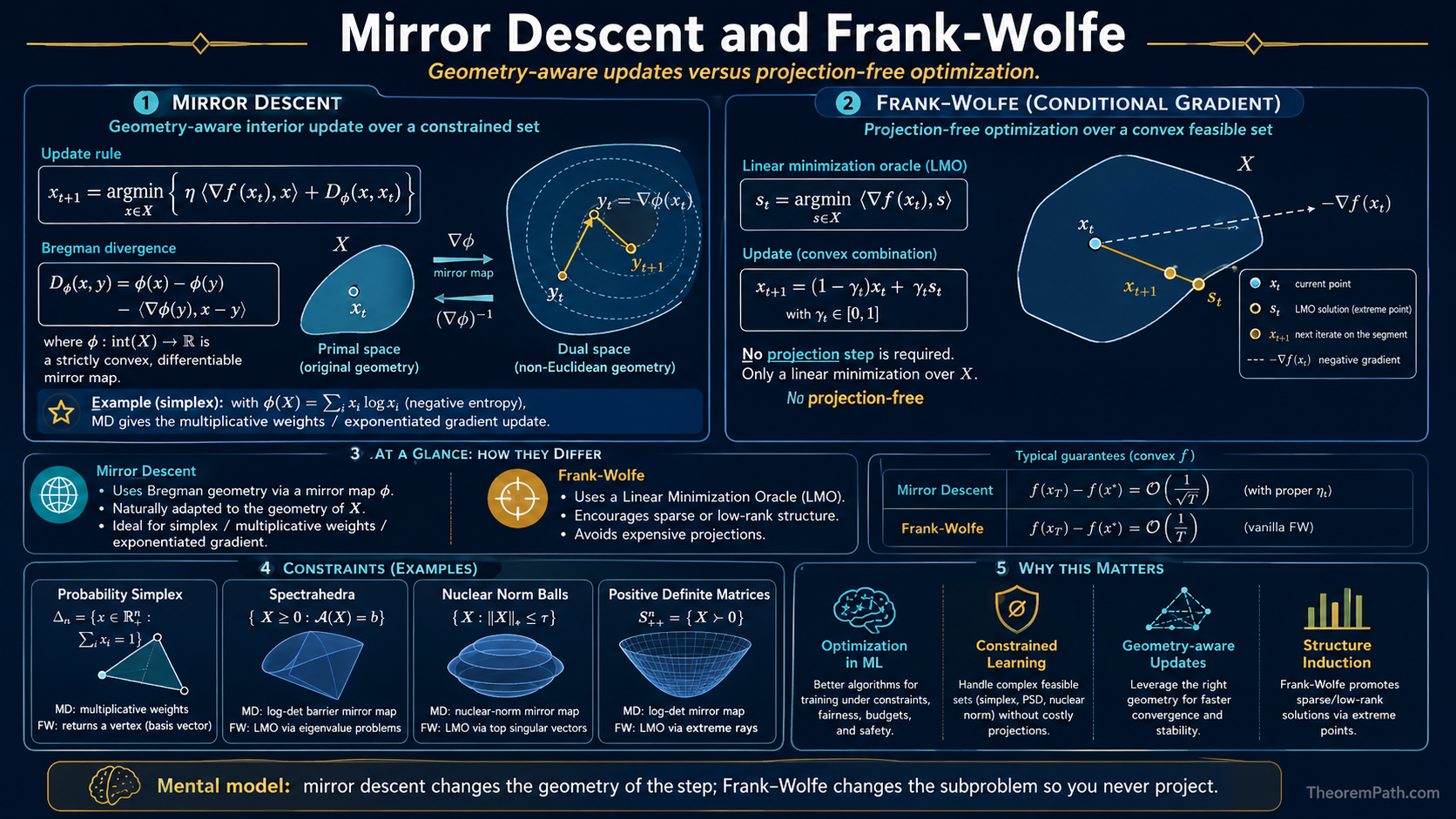
Mirror descent replaces Euclidean distance with a Bregman divergence, adapting the algorithm to the problem geometry. Frank-Wolfe goes further: it avoids projection entirely by solving a linear subproblem over the constraint set at each step.

theorem visual

Constraint Geometry Split

$Mirror descent shapes distance to the constraint geometry, while Frank-Wolfe uses a boundary oracle and moves along a feasible segment.$

Step

geometry-aware interior step

Objective

$η ⟨ \nabla f (x_{t}), x ⟩ + D_{ϕ} (x, x_{t})$

Why it helps

The mirror map reweights distance so the update respects the constraint geometry.

Bregman Divergences

Definition

Bregman Divergence $D_{ϕ} (x, y)$

Given a strictly convex, differentiable function $\phi: \mathcal{X} \to \mathbb{R}$ (the mirror map or distance-generating function), the Bregman divergence is:

$D_\phi(x, y) = \phi(x) - \phi(y) - \langle \nabla \phi(y), x - y \rangle$

This measures the gap between $\phi(x)$ and its first-order Taylor approximation at $y$ . It is always non-negative by convexity of $\phi$ , but it is generally not symmetric: $D_\phi(x, y) \neq D_\phi(y, x)$ .

Key examples:

$\phi(x) = \frac{1}{2}\|x\|_2^2$ : Bregman divergence is $D_\phi(x, y) = \frac{1}{2}\|x - y\|_2^2$ (squared Euclidean distance). Recovers standard gradient descent.
$\phi(x) = \sum_i x_i \log x_i$ (negative entropy): Bregman divergence is the KL divergence $D_{\text{KL}}(x \| y) = \sum_i x_i \log(x_i / y_i)$ . Natural for the simplex.

Mirror Descent

Definition

Mirror Descent Update

Given a convex function $f$ to minimize over a convex set $\mathcal{X}$ , the mirror descent update with step size $\eta$ is:

$x_{t+1} = \arg\min_{x \in \mathcal{X}} \left\{ \eta \langle \nabla f(x_t), x \rangle + D_\phi(x, x_t) \right\}$

Equivalently, in the "dual space": compute $\theta_{t+1} = \nabla \phi(x_t) - \eta \nabla f(x_t)$ , then "mirror back" via $x_{t+1} = \arg\min_{x \in \mathcal{X}} D_\phi(x, (\nabla \phi)^{-1}(\theta_{t+1}))$ .

The update finds the point in $\mathcal{X}$ that best balances two objectives: move in the direction of the negative gradient (minimize the linear term) while staying close to $x_t$ (minimize the Bregman divergence term).

Special cases:

Euclidean mirror map ( $\phi = \frac{1}{2}\|\cdot\|_2^2$ ): recovers projected gradient descent.
Entropic mirror map ( $\phi = \sum x_i \log x_i$ ) over the simplex: recovers the exponentiated gradient / multiplicative weights update $x_{t+1,i} \propto x_{t,i} \exp(-\eta \nabla_i f(x_t))$ .

Theorem

Mirror Descent Convergence

Statement

After $T$ iterations of mirror descent with step size $\eta = \frac{R\sqrt{2}}{L\sqrt{T}}$ , where $R^2 = \max_{x \in \mathcal{X}} D_\phi(x, x_1)$ and $\|\nabla f(x)\|_* \leq L$ for all $x$ :

$f\left(\frac{1}{T}\sum_{t=1}^T x_t\right) - f(x^*) \leq \frac{RL\sqrt{2}}{\sqrt{T}}$

This is the $O(1/\sqrt{T})$ rate for convex Lipschitz optimization.

Intuition

The rate depends on the ratio $R/\sigma$ where $R$ is the "diameter" in Bregman divergence and $L$ is the gradient bound in the dual norm. Choosing $\phi$ to match the geometry of the constraint set can make $R$ much smaller than the Euclidean diameter, giving faster effective convergence.

Proof Sketch

The standard mirror descent analysis telescopes the Bregman divergence to the optimum: $D_\phi(x^*, x_{t+1}) \leq D_\phi(x^*, x_t) - \eta(f(x_t) - f(x^*)) + \frac{\eta^2}{2\sigma}\|\nabla f(x_t)\|_*^2$ . Sum from $t = 1$ to $T$ , use $D_\phi(x^*, x_1) \leq R^2$ and $D_\phi(x^*, x_{T+1}) \geq 0$ , then optimize $\eta$ .

Why It Matters

Mirror descent with the entropic mirror map on the simplex achieves $O(\sqrt{\log d / T})$ regret, compared to $O(\sqrt{d / T})$ for projected gradient descent. The logarithmic dependence on dimension $d$ is a huge advantage in high-dimensional settings like online learning with exponentially many experts.

Failure Mode

The choice of mirror map $\phi$ is crucial. A poorly chosen $\phi$ gives a Bregman diameter $R$ that is no better (or worse) than Euclidean distance. The analysis also requires that the mirror map be strongly convex with respect to the chosen norm, which may be difficult to verify. For non-Lipschitz objectives, the rate degrades.

report a correction →

Frank-Wolfe (Conditional Gradient)

Definition

Frank-Wolfe Update

The Frank-Wolfe (conditional gradient) update for minimizing a smooth convex function $f$ over a compact convex set $\mathcal{X}$ :

Solve the linear minimization oracle (LMO): $v_t = \arg\min_{v \in \mathcal{X}} \langle \nabla f(x_t), v \rangle$
Update: $x_{t+1} = x_t + \gamma_t (v_t - x_t)$ where $\gamma_t \in [0, 1]$

The step direction $v_t - x_t$ always points into the feasible set, so no projection is needed.

The LMO is often much cheaper than projection. Over the nuclear norm ball, the LMO requires a single top singular vector computation ( $O(d^2)$ ), while projection requires a full SVD ( $O(d^3)$ ). Over polytopes, the LMO is a linear program.

Theorem

Frank-Wolfe Convergence Rate

Statement

With step sizes $\gamma_t = 2/(t+2)$ , the Frank-Wolfe algorithm satisfies:

$f(x_T) - f(x^*) \leq \frac{2L \cdot \text{diam}(\mathcal{X})^2}{T + 2}$

where $\text{diam}(\mathcal{X}) = \max_{x, y \in \mathcal{X}} \|x - y\|$ .

Intuition

The $O(1/T)$ rate is slower than the $O(1/T^2)$ of accelerated gradient descent, but each iteration only requires a linear minimization, not a projection. The trade-off is worth it when the LMO is cheap and projection is expensive.

Proof Sketch

By smoothness, $f(x_{t+1}) \leq f(x_t) + \gamma_t \langle \nabla f(x_t), v_t - x_t \rangle + \frac{L \gamma_t^2}{2}\|v_t - x_t\|^2$ . Since $v_t$ minimizes the linear term over $\mathcal{X}$ , we have $\langle \nabla f(x_t), v_t - x_t \rangle \leq \langle \nabla f(x_t), x^* - x_t \rangle \leq -(f(x_t) - f(x^*))$ by convexity. Substituting and setting $\gamma_t = 2/(t+2)$ gives the result by induction.

Why It Matters

Frank-Wolfe iterates are sparse: each iterate is a convex combination of at most $T$ vertices of $\mathcal{X}$ . This makes it natural for problems where sparse solutions are desirable (e.g., sparse optimization, low-rank matrix completion). The method also never leaves the feasible set, which matters when feasibility has physical meaning.

Failure Mode

The $O(1/T)$ rate cannot be improved in general for Frank-Wolfe without modifications (away steps, pairwise steps). The "zig-zagging" phenomenon arises when the optimum lies on the boundary of $\mathcal{X}$ , and especially on a low-dimensional face: the iterates oscillate between vertices of the active face instead of moving cleanly along it, which is precisely the case the away-step and pairwise variants are designed to fix. For strongly convex objectives, vanilla Frank-Wolfe does not achieve the linear rate that projected gradient descent achieves.

report a correction →

Common Confusions

Watch Out

Mirror descent is not just projected gradient descent with a different norm

While projected gradient descent in the $\ell_1$ norm exists, it is not the same as mirror descent with the entropic mirror map. Mirror descent changes the geometry of the update step itself (using Bregman divergence instead of squared distance), not just the metric used in the projection. The two coincide only when $\phi = \frac{1}{2}\|\cdot\|^2$ .

Watch Out

Frank-Wolfe and mirror descent solve different bottlenecks

Mirror descent replaces Euclidean distance with a better geometry but still requires a Bregman projection. Frank-Wolfe eliminates projection entirely by using a linear oracle. If projection is cheap (e.g., onto a ball), use projected gradient descent or mirror descent. If projection is expensive but linear minimization is cheap (e.g., over a polytope or nuclear norm ball), use Frank-Wolfe.

Canonical Examples

Example

Multiplicative weights from mirror descent

On the probability simplex $\Delta_d = \{x \geq 0 : \sum_i x_i = 1\}$ , use the negative entropy $\phi(x) = \sum_i x_i \log x_i$ . The mirror descent update for a linear loss $f(x) = \langle g_t, x \rangle$ gives:

$x_{t+1,i} = \frac{x_{t,i} \exp(-\eta g_{t,i})}{\sum_j x_{t,j} \exp(-\eta g_{t,j})}$

This is the multiplicative weights update, with $O(\sqrt{\log d / T})$ regret. The $\log d$ (instead of $d$ ) dependence on dimension is the key advantage over Euclidean methods.

Exercises

ExerciseCore

Problem

Verify that the Bregman divergence for $\phi(x) = \frac{1}{2}\|x\|_2^2$ is the squared Euclidean distance $\frac{1}{2}\|x - y\|_2^2$ , and that the mirror descent update reduces to the projected gradient descent update.

ExerciseAdvanced

Problem

Consider Frank-Wolfe on the $\ell_1$ ball $\{x : \|x\|_1 \leq 1\}$ in $\mathbb{R}^d$ . What does the linear minimization oracle compute? What is the sparsity of the iterate $x_T$ after $T$ steps if $x_0 = 0$ ?

References

Canonical:

Nemirovski & Yudin, Problem Complexity and Method Efficiency in Optimization (1983), Chapter 5
Frank & Wolfe, "An algorithm for quadratic programming" (1956)
Bubeck, "Convex Optimization: Algorithms and Complexity" (2015), Sections 4.2, 4.3

Current:

Jaggi, "Revisiting Frank-Wolfe: Projection-Free Sparse Convex Optimization" (2013)
Hazan, Introduction to Online Convex Optimization (2016), Chapter 5

Next Topics

Projected gradient descent: the standard projection-based approach that mirror descent generalizes
Coordinate descent: another projection-free approach for structured problems

Last reviewed: April 26, 2026

Canonical graph

Required before and derived from this topic

These links come from prerequisite edges in the curriculum graph. Editorial suggestions are shown here only when the target page also cites this page as a prerequisite.

Full prerequisite chain All derived topics

Required prerequisites

4

Convex Optimization Basicslayer 1 · tier 1
Convex Dualitylayer 2 · tier 1
Projected Gradient Descentlayer 2 · tier 2
Online Convex Optimizationlayer 3 · tier 2

Derived topics

1

Coordinate Descentlayer 2 · tier 2

Graph-backed continuations

Coordinate Descent